Game Theory

This article sketches the basic concepts of the theory of games in order to discuss some of their philosophical implications and problems.

Consider the following situation: when two hunters set out to hunt a stag and lose track of each other in the process, each hunter has to make a decision. Either she continues according to plan, hoping that her partner does likewise (because she cannot bag a deer on her own), and together they catch the deer; or she goes for a hare instead, securing a prey that does not require her partner’s cooperation, and thus abandoning the common plan. Each hunter prefers a deer shared between them to a hare for herself alone. But if she decides to hunt for deer, she faces the possibility that her partner abandons her, leaving her without deer or hare. So, what should she do? And, what will she do?

Situations like this, in which the outcome of an agent’s action depends on the actions of all the other agents involved, are called interactive. Two people playing chess is the archetypical example of an interactive situation, but so are elections, wage bargaining, market transactions, the arms race, international negotiations, and many more. Game theory studies these interactive situations. Its fundamental idea is that an agent in an interactive decision should and does take into account the deliberations of her opponents, who, in turn, take into account her deliberations. A rational agent in an interactive situation should therefore not ask: “What can I do, given what is likely to happen?” but rather: “What can I do in response to what they do, given that they have a belief about what I will do?” Based on this perspective, game theory recommends rational choices for these situations, and predicts agents’ behavior in them.

This article presents the basic tenets of game theory in a non-formal way. It then discusses two broad philosophical issues arising from the theory. First, whether the rationality concept employed by the theory is justifiable – whether it is intuitively rational to choose as the theory prescribes. Second, whether the theory can in principle be a good predictive theory of human behavior – whether it has empirical content, whether it is testable and whether there are good reasons to believe that it is true or false.

Sketch of the Theory
Game Theory as a Theory of Rationality
Game Theory as a Predictive Theory
Conclusion
References and Further Reading

1. Sketch of the Theory

Game theory belongs to a family of theories often subsumed under the umbrella term Rational Choice Theory. All these theories (in particular, decision theory, game theory and social choice theory) discuss conditions under which agents’ actions, or at least their decision to act, can be said to be rational. Depending on how these conditions are interpreted, Rational Choice theory may have a positive or a normative function: it may contribute to the prediction and explanation of agent behavior, or it may contribute to advising agents what they should do. Many of the purported functions of Rational Choice theory are controversial; as a part of it, game theory is affected by these controversies, in particular its usefulness for the social sciences. I will address some of these general issues in Section 3. However, game theory faces its own philosophical problems, and these will be the focus of this article.

Decision theory, as well as game theory, assesses the rationality of decisions in the light of preferences over outcomes and beliefs about the likelihood of these outcomes to appear. The basic difference between the two lies in the way they view the likelihood of outcomes. Decision theory treats all outcomes as exogenous events, ‘moves of nature’. Game theory, in contrast, focuses on those situations in which outcomes are determined by interactions of deliberating agents. It proposes that agents take outcomes as determined by other agents’ reasoning, and that agent therefore assess the likelihood of an outcome by trying to figure out how the other agents they interact with will reason. The likelihoods of outcomes therefore becomes “endogenous” in the sense that players take their opponents’ payoffs and rationality into account when figuring out the consequences of their strategies.

We are familiar with such reasoning from card and board games. When playing poker or chess, one must take one’s opponent’s reasoning into account in order to be successful. The player who foresees her opponent’s optimal reaction to her own move will be much more successful that the player who simply assumes that her opponent will make a certain move with a certain probability. Theoretical reflection about such parlor games are at the basis of game theory – for example, James Waldegrave’s discussion of the French card game Le Her in 1713, or von Neumann’s treatment ‘Zur Theorie der Gesellschaftsspiele’ (‘Towards a Theory of Parlor Games’) from 1928 – but today game theory has little to do with these games, and instead discusses a wide variety of social interactions. (Game theory is also applied to problems in biology and even in logic – these applications will not be discussed in this article).

The formal theory defines a game as consisting of two or more players, a set of pure strategies for each player and the players’ payoff functions. A player’s pure strategy specifies her choice for each time she has to choose in the game (which may be more than once). Players have to have at least two strategies to choose between, otherwise the game would be trivial. All players of a game together determine a consequence. Each chooses a specific strategy, and their combination (called strategy profiles) yields a specific consequence. The consequence of a strategy profile can be a material prize – for example money – but it can also be any other relevant event, like being the winner, or feeling guilt. Game theory is really only interested in the players’ evaluations of this consequence, which are specified in each players’ so-called payoff or utility function.

The part of the theory that deals with situations in which players’ choice of strategies cannot be enforced is called the theory of non-cooperative games. Cooperative game theory, in contrast, allows for pre-play agreements to be made binding (e.g. through legally enforceable contracts). This article will not discuss cooperative game theory. More specifically, it will focus – for reasons of simplicity – on non-cooperative games with two players, finite strategy sets and precisely known payoff functions.

Game theory uses two means to represent games formally: strategic form and extensive form. Commonly (though not necessarily!), these two methods of representation are associated with two different kinds of games. Extensive form games represent dynamic games, where players choose their actions in a determined temporal order. Strategic form games represent static games, where players choose their actions simultaneously.

a. Static Games

Static two-person games can be represented by m-by-n matrices, with m rows and n columns corresponding to the players’ strategies, and the entries in the squares representing the payoffs for each player for the pair of strategies (row, column) determining the square in question. As an example, figure 1 is a possible representation of the stag-hunt scenario described in the introduction.

		Col’s Choice
		C1	C2
Row’s Choice	R1	2,2	0,1
Row’s Choice	R2	1,0	1,1

Figure 1: The stag hunt

The 2-by-2 matrix of figure 1 determines two players, Row and Col, who each have two pure strategies: R1 and C1 (go deer hunting) and R2 and C2 (go hare hunting). Combining the players’ respective strategies yields four different pure strategy profiles, each associated with a consequence relevant for both players: (R1,C1) leads to them catching a deer, (R2,C1) leaves Row with a hare and Col with nothing, (R2,C2) gets each a hare and (R1,C2) leaves Row empty-handed and Col with a hare. Both players evaluate these consequences of each profile. Put informally, players rank consequences as ‘better than’ or ‘equally good as’. In the stag-hunt scenario, players have the following ranking:

Row	Col
1. (R1,C1) 2. (R2,C1); (R2,C2) 3. (R1,C2)	1. (R1,C1) 2. (R1,C2); (R2,C2) 3. (R2,C1)

Row

Col

1. (R1,C1)

2. (R2,C1); (R2,C2)

3. (R1,C2)

1. (R1,C1)

2. (R1,C2); (R2,C2)

3. (R2,C1)

Figure 2: The hunters’ respective rankings of the strategy profiles

This ranking can be quite simply represented by a numerical function u, according to the following two principles:

For all consequences X, Y: X is better than Y if and only if u(X) > u(Y)
For all consequences X, Y: X is equally good as Y if and only if u(X) = u(Y)

A function that meets these two principles (and some further requirements that are not relevant here) is called an ordinal utility function. Utility functions are used to represent players’ evaluations of consequences in games (for more on preferences and utility functions, see Grüne-Yanoff and Hansson 2006). Convention has it that the first number represents Row’s evaluation, while the second number represents Col’s evaluation. It is now easy to see that the numbers of the game in figure 1 represent the ranking of figure 2.

Note, however, that the matrix of figure 1 is not the only way to represent the stag-hunt game. Because the utilities only represent rankings, there are many ways how one can represent the ranking of figure 2. For example, the games in figures 3a-c are identical to the game in figure 1.

	C1	C2
R1	-5,-5	-7,-6
R2	-6,-7	-6,-6

Figure 3a: 3rd version of the stag hunt

	C1	C2
R1	100,100	1,99
R2	99,1	99,99

Figure 3b: 2nd version of the stag hunt

	C1	C2
R1	-5,100	-7,-99
R2	-6,1	-6,99

Figure 3c: 1st version of the stag hunt

In figure 3a, all numbers are negative, but they retain the same ranking of consequences. And similarly in figure 3b, only that here the proportional relations between the numbers (which don’t matter) are different. This should also make clear that utility numbers only express a ranking for one and the same player, and do not allow to compare different players’ evaluations. In figure 3c, although the numbers are very different for the two players, they retain the same ranking as in figure 1. Comparing, say, Row’s evaluation of (R1,C1) with Col’s evaluation of (R1,C1) simply does not have any meaning.

Note that in the stag-hunt game, agents do not gain if others lose. Everybody is better off hunting deer, and losses arise from lack of coordination. Games with this property are therefore called coordination games. They stand in stark contrast to games in which one player’s gain is the other player’s loss. Most social games are of this sort: in chess, for example, the idea of coordination is wholly misplaced. Such games are called zero-sum games. They were the first games to be treated theoretically, and the pioneering work of game theory, von Neumann and Morgenstern’s (1944) The Theory of Games and Economic Behavior concentrates solely on them. Today, many of the games discussed are of a third kind: they combine coordination aspects with conflicting aspects, so that players may at times gain from coordinating, but at other times from competing with the other players. A famous example of such a game is the Prisoners’ Dilemma, to be discussed shortly.

Players can create further strategies by randomizing over pure strategies. They can choose a randomization device (like a dice) and determine for each chance result which of their pure strategies they will play. The resultant probability distribution over pure strategies is called a mixed strategy σ. For example, Row could create a new strategy that goes as follows: toss a (fair) coin. Play R1 if heads, and R2 if tails. Because a fair coin lands heads 50% of the time, such a mixed strategy is denoted σ_R = (0.5,0.5). As there are no limits to the number of possible randomization devices, each player can create an infinite number of mixed strategies for herself. The players’ evaluation of mixed strategies profiles is represented by the expected values of the corresponding pure-strategy payoffs. Such an expected value is computed as the weighted average of the pure-strategy payoffs, and the weights are the probabilities with which each strategy is played. For example, if Row in figure 1 plays her mixed strategy σ_R = (0.5,0.5), and Col plays a strategy σ_C = (0.8,0.2), then Row’s expected utility will be computed by:

u_R(σ_R,σ_C) = 0.5(0.8×2 + 0.2×0) + 0.5(0.8×1 + 0.2×1) = 1.3

With the same mixed strategies, Col’s expected utility, u_C(σ_R,σ_C) = 1. For the payoffs of mixed strategy to be computable, the utility function has to carry cardinal information. Now it is also important how much a player prefers a consequence X to a consequence Y, in comparison to another pair of consequences X and Z. Because mixed strategies are a very important concept in game theory, it is generally assumed that the utility functions characterizing the payoffs are cardinal. However, it is important to note that cardinal utilities also do not allow making interpersonal comparisons. In fact, such interpersonal comparisons play no role in standard game theory at all.

Solution Concepts

Representing interactive situations in these highly abstract games, the objective of game theory is to determine the outcome or possible outcomes of each game, given certain assumptions about the players. To do this is to solve a game. Various solution concepts have been proposed. The conceptually most straightforward solution concept is the elimination of dominated strategies. Take the game of figure 4 (which, take note, differs from the stag-hunt game in its payoffs). In this game, no matter what Col chooses, playing R2 gives Row a higher payoff. If Col plays C1, Row is better off playing R2, because she can obtain 3 utils instead of two. If Col plays C2, Row is also better off playing R2, because she can obtain 1 utils instead of none. Similarly for Col: no matter what Row chooses, playing C2 gives her a higher payoff. This is what is meant by saying that R1 and C1 are strictly dominated strategies.

	C1	C2
R1	2,2	0,3
R2	3,0	1,1

Figure 4: The Prisoners’ Dilemma

More generally, a player A’s pure strategy is strictly dominated if there exists another (pure or mixed) strategy for A that has a higher payoff for each of A’s opponent’s strategies. To solve a game by eliminating all dominated strategies is based on the assumption that players do and should choose those strategies that are best for them, in this very straightforward sense. In cases like in figure 4, where each player has only one non-dominated strategy, the elimination of dominated strategies is a straightforward and plausible solution concept. However, there are many games, which do not have any dominated strategies, as for example the stag-hunt game or the zero-sum game of figure 5.

Recall that in a zero sum game, one player’s payoff is exactly the inverse of that of the other player. For example, figure 5 shows Row’s payoffs, while Col’s payoffs are the negative of Row’s payoffs.

	C1	C2	C3
R1	1	3	6
R2	7	5	5
R3	3	4	10

Figure 5: A zero-sum game

Von Neumann and Morgenstern argued for the Minimax Rule as the solution concept for zero-sum games. In these games, they suggest, each player makes the following consideration: ‘my adversary tries to get out of the play as much as possible. Her gain is my loss. So I better look for how much I minimally get out of each option and try to make this amount as large as possible. If this is reasonable, then my adversary will do the same. Since my maximizing my minimum is best against her maximizing her minimum, I should stick to my choice’. The minimax solution therefore recommends that Row choose the strategy with the highest minimum, while Col choose a strategy with the lowest maximum. Thus, in figure 5, Row chooses R2, as it has the highest minimal payoff for her, and Col chooses C2, as it has the lowest maximal payoff for Row (and hence the highest minimal payoff for her).

Unfortunately, there are many non-zero-sum games without dominated strategies, for example the game of figure 6.

	C1	C2	C3
R1	3,4	2,5	1,3
R2	4,8	1,2	0,9

Figure 6: A game without dominated strategies

For these kinds of games, the Nash equilibrium solution concept offers greater versatility than dominance or maximin (as it turns out, all maximin solutions are also Nash equilibria). In contrast to dominated strategy elimination, the Nash equilibrium applies to strategy profiles, not to individual strategies. Roughly, a strategy profile is in Nash equilibrium if none of the players can do better by unilaterally changing her strategy. Take the example of matrix 6. Consider the strategy profile (R1,C1). If Row knew that Col would play C1, then she would play R2 because that’s the best she can do against C1. On the other hand, if Col knew that Row would play R1, he would play C2 because that’s the best he can do against R1. So (R1, C1) is not in equilibrium, because at least one player (in this case both) is better off by unilaterally deviating from it. Similarly for (R1, C3), (R2, C1), (R2,C2) and (R2, C3): in all these profiles, one of the players can improve her or his lot by deviating from the profile. Only (R1, C2) is a pure strategy Nash equilibrium – neither player is better off by unilaterally deviating from it.

There are games without a pure strategy Nash equilibrium, as matrix 7 shows. The reader can easily verify that each player has an incentive to deviate, whichever pure strategy the other chooses.

	C1	C2
R1	1,-1	-1,1
R2	-1,1	1,-1

Figure 7: Matching pennies

However, there is an equilibrium involving mixed strategies. Randomizing between the two strategies, assigning equal probability to each, yields a payoff of 0.5(0.5×1+0.5x-1)+0.5(0.5×1+0.5x-1) = 0 for both players. As mutually best responses, these mixed strategies constitute a Nash equilibrium. As one of the fundamental results of game theory, it has been shown that every finite static game has a mixed-strategy equilibrium (Nash 1950). Many games have several Nash equilibria. Take for example figure 1. There, neither player has an incentive to deviate from (R1, C1), nor to deviate from (R2, C2). Thus both strategy profiles are pure-strategy Nash equilibria. With two or more possible outcomes, the equilibrium concept loses much of its appeal. It no longer gives an obvious answer to the normative, explanatory or predictive questions game theory sets out to answer. The assumption that one specific Nash equilibrium is played relies on there being some mechanism or process that leads all the players to expect the same equilibrium.

Schelling’s (1960) theory of focal points suggests that in some “real-life” situations players may be able to coordinate on a particular equilibrium by using information that is abstracted away by the strategic form. Examples of information that has such focal power may be the names of strategies or past common experiences of the players. Little systematic work exists on the “focalness” of various strategies, as they depend on the players’ cultural and personal backgrounds. Mainstream game theory has never incorporated these concepts into the formal structure of the theory (for exceptions, see Bacharach 1993, Sugden 1995).

A focal point that might evade such context-dependence is Pareto-dominance, if pre-play communication is allowed. An equilibrium is Pareto-dominant over another if it makes everybody at least as well off and makes at least one person better off. This is the case in the game of figure 1: (R1, C1) makes both players better off than (R2, C2). The intuition for this focal point is that, even though the players cannot commit themselves to play the way they claim they will, the pre-play communication lets the players reassure one another about the low risk of playing the strategy of the Pareto-dominant equilibrium. Although pre-play communication may make the Pareto-dominant equilibrium more likely in the stag-hunt game, it is not clear that it does so in general. Many other selection mechanisms have been proposed that use clues derivable from the game model alone. These mechanisms are however too complex to be discussed here.

As it will become clearer in Section 2b, the assumptions underlying the application of the Nash concept are somewhat problematic. The most important alternative solution concept is that of rationalizability, which is based on weaker assumptions. Instead of relying on the equilibrium concept, rationalizability selects strategies that are “best” from the players’ subjective point of view. Players assign a subjective probability to each of the possible strategies of their opponents, instead of postulating their opponents’ choices and then finding a best response to it, as in the Nash procedure. Further, knowing their opponent’s payoffs, and knowing they are rational, players expect others to use only strategies that are best responses to some belief they might have about themselves. And those beliefs in turn are informed by the same argument, leading to an infinite regress of the form: “I’m playing strategy σ1 because I think player 2 is using σ2, which is a reasonable belief because I would play it if I were player 2 and I thought player 1 was using σ1’, which is a reasonable thing for player 2 to expect because σ1’ is a best response to σ2’…”. A strategy is rationalizable for a player if it survives infinitely repeated selections as a best response to some rational belief she might have about the strategies of her opponent. A strategy profile is rationalizable if the strategies contained in it are rationalizable for each player. It has been shown that every Nash equilibrium is rationalizable. Further, the set of rationalizable strategies is nonempty and contains at least one pure strategy for each player (Bernheim 1984, Pearce 1984). The problem with rationalizability is thus not its applicability; rather, there are too many rationalizable strategies, so that the application of rationalizability often does not provide a clear answer to the advisory and predictive questions posed to game theory.

b. Dynamic Games

In static games discussed above, players choose their actions simultaneously. Many interactive situations, however, are dynamic: a player chooses before others do, knowing that the others choices will be influenced by his observable choice. Players who choose later will make their choices dependent on their knowledge of how others have chosen. Chess is a typical example of such a dynamic interactive situation (although one, as will be seen, that is far too complex to explicitly model it). Game theory commonly represents these dynamic situations in extensive form. This representation makes explicit the order in which players move, and what each player knows when making each of his decisions.

The extensive form consists of six elements. First, the set of players is determined. Each player is indexed with a number, starting with 1. Second, it is determined who moves when. The order of moves is captured in a game tree, as illustrated in figure 8. A tree is a finite collection of ordered nodes x (This index is for instructive purposes only. Commonly, nodes are only indexed with the number of the player choosing at this node). Each tree starts with one (and only one!) initial node, and grows only ‘down’ and never ‘up’ from there. The nodes that are not predecessors to any others are called terminal nodes, denoted z1-z4 in figure 8. All nodes but the terminal ones are labeled with the number of that player who chooses at this node. Each z describes a complete and unique path through the tree from the initial to one final node.

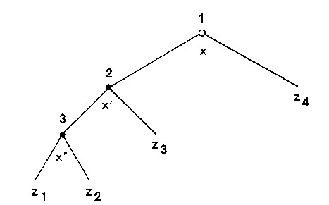
Figure 8: A game tree

Third, the payoffs for all players are assigned (as an list of utility numbers: first player’s utility in the first place, etc.) to the terminal nodes. An illustration is given in figure 8. The utility functions of each player have to satisfy the same requirements as those in static games. Fourth, for each player at each node, a finite set of actions is specified, labeled with capital letters in figure 8. Each action leads to one (and only one) non-initial node. Fifth, it is determined what each player knows about her position in the game when she makes her choice. Her knowledge is represented by a partition of the nodes of the tree, called the information set. If the information set contains, say, nodes x and x’, this means that the player who is choosing an action at x is uncertain whether she is at x or at x’. To avoid inconsistencies, information sets can contain only nodes at which the same player chooses, and only nodes where the same player has the same actions to choose from. In figure 9, an information set containing more than one node is represented as a dotted line between those nodes (Information sets that contain only one node are usually not represented). Games that contain only singleton information sets are called games of perfect information: all agents know where they are at all nodes of the game. Further, it is commonly assumed that agents have perfect recall: they neither forget what they once knew, nor what they have chosen.

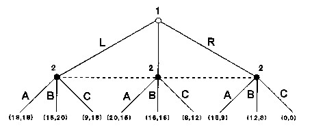
Figure 9: A game of imperfect information

Sixth and last, when a game involves chance moves, the probabilities are displayed in brackets, as in the game of figure 10. There, a chance move (by an imagined player called N like “Nature’) determines the payoffs for both players. Player 1 then plays L or R. Player 2 observes player 1’s action, but does not know whether he is at x or x’ (if player 1 chose L) nor whether he is at y or y’ (if player 1 chose R). In other words, player 2 faces a player whose payoffs he does not know. All he knows is that player 1 can be either of two types, distinguished by the respective utility function.

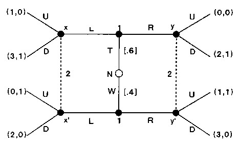
Figure 10: A game of incomplete information

Games such as that in figure 10 will not be further discussed in this article. They are games of incomplete information, where players do not know their and other players’ payoffs, but only have probability distributions over them.

Extensive-form games can be represented as strategic-form games. While in extensive-form interpretation, the players “wait” until their respective information set is reached to make a decision, in the strategic-form interpretation they make a complete contingency plan in advance. Figure 11 illustrates this transformation. Player 1, who becomes “Row’, has only two strategies to choose from. Player 2, who becomes “Col’, has to decide in advance for both the case where player 1 chooses U and where she chooses D. His strategies thus contain two moves each: for example, (L,R) means that he plays L after U and R after D.

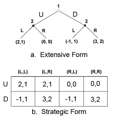
Figure 11: Extensive form reduced to strategic form

A similar terminology as in strategic-form games applies. A pure strategy for a player determines her choice at each of her information sets (That is, a strategy specifies all the past and future moves of an agent. Seen from this perspective, one may legitimately doubt whether extensive games really capture the dynamics of interaction to any interesting extent). A behavior strategy specifies a probability distribution over actions at each information set. For games of perfect recall, behavior strategies are equivalent to mixed strategies known from strategic-form games (Kuhn 1953).

Solution Concepts

Given that the strategic form can be used to represent arbitrarily complex extensive-form games, the Nash equilibrium can also be applied as a solution concept to extensive form games. However, the extensive form provides more information than the strategic form, and on the basis of that extra information, it is sometimes possible to separate the “reasonable” from the “unreasonable” Nash equilibria. Take the example from figure 11. The game has three Nash equilibria, which can be identified in the game matrix: (U, (L,L)); (D, (L,R)) and (D, (R,R)). But the first and the third equilibria are suspect, when one looks at the extensive form of the game. After all, if player 2’s right information set was reached, the he should play R (given that R gives him 3 utils while L gives him only –1 utils). But if player 2’s left information set was reached, then he should play L (given that L gives him 2 utils, while R gives him only 0 utils). Moreover, player 1 should expect player 2 to choose this way, and hence she should choose D (given that her choosing D and player 2 choosing R gives her 2 utils, while her choosing U and player 2 choosing L gives her only 1 util). The equilibria (U, (L,L)) and (D, (R,R)) are not “credible’, because they rely on an “empty threat” by player 2. The threat is empty because player 2 would never wish to carry out either of them. The Nash equilibrium concept neglects this sort of information, because it is insensitive to what happens off the path of play.

To identify “reasonable” Nash equilibria, game theorists have employed equilibrium refinements. The simplest of these is the backward-induction solution that applies to finite games of perfect information. Its rational was already used in the preceding paragraph. “Zermelo’s algorithm” (Zermelo 1913) specifies its procedure more exactly: Since the game is finite, it has a set of penultimate nodes – i.e. nodes whose immediate successors are terminal nodes. Specify that the player, who can move at each such node, chooses whichever action that leads to the successive terminal node with the highest payoff for him (in case of a tie, make an arbitrary selection). So in the game of figure 11, player 2’s choices R if player 1 chooses U and L if player 1 chooses D can be eliminated:

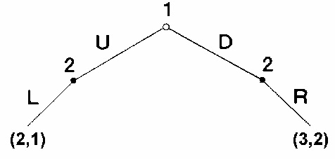
Figure 11a: First step of backward induction

Now specify that each player at those nodes, whose immediate successors are penultimate nodes, choose the action that maximizes her payoff over the feasible successors, given that the players at the penultimate nodes play as we have just specified. So now player 1’s choice U can be eliminated:

Figure 11b: Second step of backward induction

Then roll back through the tree, specifying actions at each node (not necessary for the given example anymore, but one gets the point). Once done, one will have specified a strategy for each player, and it is easy to check that these strategies form a Nash equilibrium. Thus, each finite game of perfect information has a pure-strategy Nash equilibrium.

Backward induction fails in games with imperfect information. In a game like in figure 12, there is no way to specify an optimal choice for player 2 in his second information set, without first specifying player 2’s belief about the previous choice of player 1. Zermelo’s algorithm is inapplicable because it presumes that such an optimal choice exists at every information set given a specification of play at its successors.

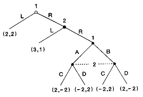
Figure 12: A game not solvable by backward induction

However, if one accepts the argument for backward induction, the following is also convincing. The game beginning at player 1’s second information set is a simultaneous-move game identical to the one presented in figure 7. The only Nash equilibrium of this game is a mixed strategy with a payoff of 0 for both players (as argued in Section 1a). Using the equilibrium payoff as player 2’s payoff to choose R, it is obvious that player 2 maximizes his payoff by choosing L, and that player 1 maximizes her payoff by choosing R. More generally, an extensive form game can be analyzed into proper subgames, each of which satisfies the definition of extensive-form games in their own right. Games of imperfect information can thus be solved by replacing a proper subgame with one of its Nash equilibrium payoffs (if necessary repeatedly), and performing backward induction on the reduced tree. This equilibrium refinement technique is called subgame perfection.

Repeated Games

Repeated games are a special kind of dynamic game. They proceed in temporal stages, and players can observe all players’ play of these previous stages. At the end of each stage, however, the same structure repeats itself. Let’s recall the static game of figure 4. As discussed in the previous section, it can be equivalently represented as an extensive game where player 2 does not know at which node he is.

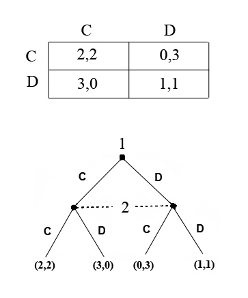
Figure 13: Equivalent Static and Extensive Games

All that changed from the original game from figure 4 is the nomination of the players (Row becomes 1 and Col becomes 2) and the strategies (C and D). A repetition of this game is shown in figure 14. Instead of the payoff matrices, at each of terminal nodes of the original static game, the same game starts again. The payoffs accumulate over this repetition: while in the static game, the strategy profile (D,D) yields (1,1), the strategy profile ((D,D),(D,D)) in figure 14 yields (2,2). These payoffs are written at the terminal nodes of the last repetition game.

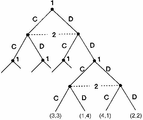
Figure 14: A repeated Prisoners’ Dilemma

If a repeated game ends after a finite number of stages, it is solved by subgame perfection. Starting with the final subgames, the Nash equilibrium in each is (D,D). Because the payoffs are accumulative, the preference structure within each subgame does not change (recall from Section 1a that only ordinal information is needed here). Thus for each subgame at any stage of the repetition, the Nash equilibrium will be (D,D). Therefore, for any number of finite repetitions of the game from figure 4, subgame perfection advises both players to always play D.

All this changes dramatically, if the game is repeated indefinitely. The first thing that needs reinterpretation are the payoffs. Any positive payoff, whether large or small, would be infinitely large if they just summed up over indefinitely many rounds. This would obliterate any interesting concept of an indefinitely repeated game. Fortunately, there is an intuitive solution: people tend to value present benefits higher than those in the distant future. In other words, they discount the value of future consequences by the distance in time by which these consequences occur. Hence in indefinitely repeated games, players’ payoffs are specified as the discounted sum of what each player wins at each stage.

The second thing that changes with indefinitely repeated game is that the solution concept of subgame perfection does not apply, because there is no final subgame at which the solution concept could start. Instead, the players may reason as follows. Player 1 may tell player 2 that she is well disposed towards him, relies on his honesty, and will trust him (i.e. play C) until proven wrong. Once he proves to be untrustworthy, she will distrust him (i.e. play D) forever. In the infinitely repeated game, player 2 has no incentive to abuse her trust if he believes her declaration. If he did, he would make a momentary gain from playing D while his opponent plays C. This would be followed, however, by him forever forgoing the extra benefit from (C,C) in comparison to (D,D). Unless player 2 has a very high discount rate, the values the present gain from cheating will be offset by the future losses from non-cooperating. More generally, the folk theorem shows that in infinitely repeated games with low enough discounting of the future, any strategy that give each player more than the worst payoff the others can force him to take is sustainable as an equilibrium (Fudenberg and Maskin 1986). It is noteworthy that for the folk theorem to apply, it is sufficient that players do not know when a repeated game ends, and have a positive belief that it may go on forever. It is more appropriate to speak of indefinitely repeated games, than of infinitely repeated ones, as the former does not conflict with the intuition that humans cannot interact infinitely many times.

c. The Architecture of Game Theory

From a philosophy of science perspectives, game theory has an interesting structure. Like many other theories, it employs highly abstract models, and it seeks to explain, to predict and to advice on phenomena of the real world by a theory that operates through these abstract models. What is special about game theory, however, is that this theory does not provide a general and unified mode of dealing with all kinds of phenomena, but rather offers a ‘toolbox’, from which the right tools must be selected.

As discussed in the two preceding sections, game theory consists of game forms (the matrices and trees), and a set of propositions (the ‘theory proper’) that defines what a game form is and provides solution concepts that solve these models. Game theorists often focus on the development of the formal apparatus of the theory proper. Their interest lies in proposing alternative equilibrium concepts or proving existing results with fewer assumptions, not in representing and solving particular interactive situations. “Game theory is for proving theorems, not for playing games” (Reinhard Selten, quoted in Goeree and Holt 2001, 1419).

Although they habitually employ labels like ‘players’, ‘strategies’ or ‘payoffs’, the game forms that the theory proper defines and helps solving are really only abstract mathematical objects, without any link to the real world. After all, only very few social situations come with labels like ‘strategies’ or ‘rules of the game’ attached. What is needed instead is an interpretation of a real-world situation in terms of the formal elements provided by the theory proper, so that it can be represented by a game form. In many cases, this is where all the hard work lies: to construct a game form that captures the relevant aspects of a real social phenomenon. To acquire an interpretation, the game forms are complemented with an appropriate story (Morgan 2005) or model narrative. As regularly exemplified in textbooks, this narrative may be purely illustrative: it provides (in non-formal terms) a plausible account of an interactive situation, whose salient features can be represented by the formal tools of game theory. A good example of such a narrative is given by Selten when discussing the ‘Chain Store Paradox’:

A chain store, also called player A, has branches in 20 towns, numbered from 1 to 20. In each of these towns there is a potential competitor, a small businessman who might raise money at the local bank in order to establish a second shop of the same kind. The potential competitor at town k is called player k. […]
Just now none of the 20 small businessmen has enough owned capital to be able to get a sufficient credit from the local bank but as time goes on, one after the other will have saved enough to increase his owned capital to the required amount. This will happen first to player 1, then to player 2, etc. As soon as this time comes for player k, he must decide whether he wants to establish a second shop in his town or whether he wants to use his owned capital in a different way. If he chooses the latter possibility, he stops being a potential competitor of player A. If a second shop is established in town k, then player A has to choose between two price policies for town k. His response may be ‘cooperative’ or ‘aggressive’. The cooperative response yields higher profits in town k, both for player A and for player k, but the profits of player A in town k are even higher if player k does not establish a second shop. Player k’s profits in case of an aggressive response are such that it is better for him not to establish a second shop if player A responds in this way. (Selten 1978, 127).

The narrative creates a specific, if fictional, context that is congruent with the structure of dynamic form games. The players are clearly identifiable, and the strategies open to them are specified. The story also determines the material outcomes of each strategy combination, and the players’ evaluation of these outcomes. The story complements a game form of the following sort:

Figure 15: One step in the Chain store’s paradox

Game form and model narrative together constitute a model of a possible real-world situation. The model narrative fulfills two crucial functions in the model. If the game form is given first, it interprets this abstract mathematical object as a possible situation; if a real-world phenomenon is given first, it accounts for the phenomenon in such a way that it can be represented by a game form, which in turn can be solved by the theory proper.

The architecture of game theory is summarized in figure 16:

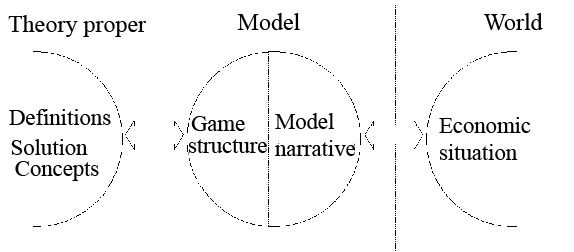
Figure 16: The architecture of game theory (Grüne-Yanoff and Schweinzer 2008)

The theory proper (on the left hand side of Figure 16) specifies the concept of a game, it provides the mathematical elements that are needed for the construction of a game form, and it offers solution concepts for the thus constructed game forms. The game form (left half of the central circle) is constructed from elements of the theory proper. The model narrative (the right half of the central circle) provides an account of a real or hypothetical economic situation. Its account of the situation interprets the game form.

As discussed in the previous sections, however, a specified game form can be solved by different solution concepts. Sometimes, as in the case of minimax and Nash equilibrium for zero-sum games, the reasoning behind the solution concepts is different, but the result is always the same. In other cases, in particular when equilibrium refinements are applied, applying different solution concepts to the same game form yields different results. As will be seen in Section 2e, this is also the case with the chain-store paradox. The reason for this ambiguity is that the application of many solution concepts requires information that is not contained in the game form. Instead, the information needed is found in an appropriate account of the situation – i.e. in the model narrative. Thus the model narrative takes on a third crucial function in game theory: it supports the choice of the appropriate solution concept for a specific game (Grüne-Yanoff and Schweinzer 2008).

This observation about the architecture of game theory and the role of informal model narratives in it has two very important implications. First, it becomes clear that game theory does not offer a universal notion of rationality, but rather offers a menu of tools to model specific situations at varying degrees and kinds of rationality. Ultimately, it is the modeler who judges on her own intuitions which kind of rationality to attributed to the interacting agents in a given situation. This opens up the discussion about the various intuitions that lie behind the solution concepts, the possibility of mutually inconsistent intuitions, and the question whether a meta-theory can be constructed that unifies all these fragmentary intuitions. Some of these issues will be discussed in Section 2.

The second implication of this observation concerns the status of game theory as a positive theory. Given its multi-layer architecture, any disagreement of prediction and observation can be attributed to a mistake either in the theory, the game form or the model narrative. This then raises the question how to test game theory, and whether game theory is refutable in principle. These questions will be discussed in Section 3.

2. Game Theory as a Theory of Rationality

Game theory has often been interpreted as a part of a general theory of rational behavior. This interpretation was already in the minds of game theories’ founders, who wrote in their Theory of Games and Economic Behavior:

We wish to find the mathematically complete principles which define “rational behavior” for the participants in a social economy, and to derive from them the general characteristics of that behavior (von Neumann and Morgenstern 1944, 31).

To interpret game theory as a theory of rationality means to give it a prescriptive task: it recommends what agents should do in specific interactive situations, given their preferences. To evaluate the success of this rational interpretation of game theory means to investigate its justification, in particular the justification of the solution concepts it proposes. That human agents ought to behave in such and such a way of course does not mean that they will do so; hence there is little sense in testing rationality claims empirically. The rational interpretation of game theory therefore needs to be distinguished from the interpretation of game theory as a predictive and explanatory theory. The solution concepts are either justified by identifying sufficient conditions for them, and showing that these conditions are already accepted as justified; or they can be justified directly by compelling intuitive arguments.

a. Sufficient Epistemic Conditions for Solution Concepts

One way to investigate game theoretic rationality is to reduce its solution concepts to the more intuitively understood notion of rationality under uncertainty in decision theory. By clearly stating the decision theoretic conditions agents have to satisfy in order to choose in accordance with game theoretic solution concepts, we obtain a better understanding of what game theory requires, and are thus able to assess criticism against it more clearly.

Recall that the various solution concepts presented in Section 1 advise how to choose one’s action rationally when the outcome of one’s choice depends on the actions of the other players, who in turn base their choices on the expectation of how one will choose. The solution concepts thus not only require the players to choose according to maximization considerations; they also require the agent to maximize their expected utilities on the basis of certain beliefs. Most prominently, these beliefs include their expectations about what the other players expect of them, and their expectations what the other players will choose on the basis of these expectations. These conditions are often not made explicit when people discuss game theory; however, without fulfilling them, players cannot be expected to choose in accord with specific solution concepts. To make these conditions on the agent’s knowledge and beliefs explicit will thus further our understanding what is involved in the solution concepts. In addition, if these epistemic conditions turn out to be justifiable, one would have achieved progress in justifying the solution concepts themselves. This line of thought has in fact been so prominent that the interpretation of game theory as a theory of rationality has often been called the eductive or epistemic interpretation. In the following, the various solution concepts discussed with respect to their sufficient epistemic conditions, and the conditions are investigated with regard to their acceptability.

For the solution of eliminating dominated strategies, nothing is required beyond the rationality of the players and their knowledge of their own strategies and payoffs. Each player can rule out her dominated strategies on the basis of maximization considerations alone, without knowing anything about the other player. To the extent that maximization considerations are accepted, this solution concept is therefore justified.

The case is more complex for iterated elimination of dominated strategies (this solution concept was not explained before, so don’t be confused. It fits in most naturally here). In the game matrix of figure 17, only Row has a dominated strategy, R1. Eliminating R1 will not yield a unique solution. Iterated elimination allows players to consecutively eliminate dominated strategies. However, it requires stronger epistemic conditions.

	C1	C2	C3
R1	3,2	1,3	1,1
R2	5,4	2,1	4,2
R3	4,3	3,2	2,4

Figure 17: A game allowing for iterated elimination of dominated strategies

If Col knows that Row will not play R1, she can eliminate C2 as a dominated strategy, given that R1was eliminated. But to know that, Col has to know:

Row’s strategies and payoffs
that Row knows her strategies and payoffs
that Row is rational

Let’s assume that Col knows i.-iii., and that he thus expects Row to have spotted and eliminated R1 as a dominated strategy. Given that Row knows that Col did this, Row can now eliminate R3. But for her to know that Col eliminated C2, she has to know:

Row’s (i.e. her own) strategies and payoffs
that she, Row, is rational
that Col knows i.-ii.
Col’s strategies and payoffs
that Col knows her strategies and payoffs
that Col is rational

Lets look at the above epistemic conditions a bit more closely. i. is trivial, as she has to know her own strategies and payoffs even for simple elimination. For simple elimination, she also has to be rational, but she does not have to know it – hence ii. If Row knows i. and ii., she knows that she would eliminate R1. Similarly, if Col knows i. and ii., he knows that Row would eliminate R1. If Row knows that Col knows that she would eliminate R1, and if Row also knows iv.-vi., then she knows that Col would eliminate C2. In a similar fashion, if Col knows that Row knows i.-vi., she will know that Row would eliminate R3. Knowing this, he would eliminate C3, leaving (R2,C1) as the unique solution of the game.

Generally, iterated elimination of dominated strategy requires that each player knows the structure of the game, the rationality of the players and, most importantly, that she knows that the opponent knows that she knows this. The depth of one player knowing that the other knows, etc. must be at least as high as the number of iterated elimination necessary to arrive at a unique solution. Beyond that, no further “he knows that she knows that he knows…” is required. Depending on how long the chain of iterated eliminations becomes, the knowledge assumptions may become difficult to justify. In long chains, even small uncertainties in the players’ knowledge may thus put the justification of this solution concept in doubt.

From the discussion so far, two epistemic notions can be distinguished. If all players know a proposition p, one says that they have mutual knowledge of p. As the discussion of iterated elimination showed, mutual knowledge is too weak for some solution concepts. For example, condition iii insists that Row not only know her own strategies, but also knows that Col knows. In the limit, this chain of one player knowing that the other knows that p, that she knows that he knows that she knows that p, etc. is continued ad infinitum. In this case, one says that players have common knowledge of the proposition p. When discussing common knowledge, it is important to distinguish of what the players have common knowledge. Standardly, common knowledge is of the structure of the game and the rationality of the players. As figure 18 indictates, this form of common knowledge is sufficient for the players to adhere to solutions provide by rationalizability.

Solution Concept	Structure of the Game	Rationality	Choices or Beliefs
Simple Elimination of Dominated Strategies	Each player knows her payoffs	Fact of rationality	—
Iterated Elimination of Dominated Strategies	Knowledge of the degree of iteration	Knowledge of the degree of iteration	—
Rationalizability	Common knowledge	Common knowledge	—
Pure-Strategy Nash Equilibrium	—	Fact of rationality	Mutual knowledge of choices
Mixed-Strategy Equilibrium in Two-Person Games	Mutual knowledge	Mutual knowledge	Mutual knowledge of beliefs

Figure 18: Epistemic requirements for solution concepts (adapted from Brandenburger 1992)

As figure 18 further indicates, sufficient epistemic conditions for pure-strategy Nash equilibria are even more problematic. Common knowledge of the game structure or rationality is neither necessary nor sufficient, not even in conjunction with epistemic rationality. Instead, it is required that all players know what the others will choose (in the pure-strategy case) or what the others will conjecture all players will be choosing (in the mixed-strategy case). This is an implausibly strong requirement. Players commonly do not know how their opponents will play. If there is no argument how players can reliably obtain this knowledge from less demanding information (like payoffs, strategies, and common knowledge thereof) then the analysis of the epistemic conditions would put into doubt whether players will reach Nash equilibrium. Note, however, that these epistemic conditions are sufficient, not necessary. Formally, nobody has been able to establish alternative epistemic conditions that are sufficient. But by discussing alternative reasoning processes, some authors have at least provided arguments for the plausibility that player soften reach Nash equilibrium. Some of these arguments will be discussed in the next section. (For further discussion of epistemic conditions of solution concepts, see Bicchieri 1993, chapter 2).

b. Nash Equilibrium in One-Shot Games

The Nash equilibrium concept is often seen as “the embodiment of the idea that economic agents are rational; that they simultaneously act to maximize their utility” (Aumann 1985, 43). Particularly in the context of one-shot games, however, doubts remain about the justifiability of this particular concept of rationality. It seems reasonable to claim that once the players have arrived at an equilibrium pair, neither has any reason for changing his strategy choice unless the other player does too. But what reason is there to expect that they will arrive at one? Why should Row choose a best reply to the strategy chosen by Col, when Row does not know Col’s choice at the time she is choosing? In these questions, the notion of equilibrium becomes somewhat dubious: when scientists say that a physical system is in equilibrium, they mean that it is in a stable state, where all causal forces internal to the system balance each other out and so leave it “at rest” unless it is disturbed by some external force. That understanding cannot be applied to the Nash equilibrium, when the equilibrium state is to be reached by rational computation alone. In a non-metaphorical sense, rational computation simply does not involve causal forces that could balance each other out. When approached from the rational interpretation of game theory, the Nash equilibrium therefore requires a different understanding and justification. In this section, two interpretations and justifications of the Nash equilibrium are discussed.

Self-Enforcing Agreements

Often, the Nash equilibrium is interpreted as a self-enforcing agreement. This interpretation is based on situations in which agents can talk to each other, and form agreements as to how to play the game, prior to the beginning of the game, but where no enforcement mechanism providing independent incentives for compliance with agreements exists. Agreements are self-enforcing if each player has reasons to respect them in the absence of external enforcement.

It has been argued that self-enforcing agreement is neither necessary nor sufficient for Nash equilibrium. That it is not necessary is quite obvious in games with many Nash equilibria. For example, the argument for focal points, as discussed in Section 1a, states that only Nash equilibria that have some extra ‘focal’ quality are self-enforcing. It also has been argued that Nash equilibria are not sufficient. Risse (2000) argues that the notion of self-enforcing agreements should be understood as an agreement that provides some incentives for the agents to stick to it, even without external enforcement. He then goes on to argue that there are such self-enforcing agreements that are not Nash equilibria. Take for example the game in figure 19.

	C1	C2
R1	0,0	4,2
R2	2,4	3,3

Figure 19

Lets imagine the players initially agreed to play (R2, C2). Now both have serious reasons to deviate, as deviating unilaterally would profit either player. Therefore, the Nash equilibria of this game are (R1,C2) and (R2,C1). However, in an additional step of reflection, both players may note that they risk ending up with nothing if they both deviate, particularly as the rational recommendation for each is to unilaterally deviate. Players may therefore prefer the relative security of sticking to the agreed-upon strategy. They can at least guarantee 2 utils for themselves, whatever the other player does, and this in combination with the fact that they agreed on (R2, C2) may reassure them that their opponent will in fact play strategy 2. So (R2, C2) may well be a self-enforcing agreement, but it nevertheless is not a Nash equilibrium.

Last, the argument from self-enforcing agreements does not account for mixed strategies. In mixed equilibria all strategies with positive probabilities are best replies to the opponent’s strategy. So once a player’s random mechanism has assigned an action to her, she might as well do something else. Even though the mixed strategies might have constituted a self-enforcing agreement before the mechanism made its assignment, it is hard to see what argument a player should have to stick to her agreement after the assignment is made (Luce ad Raiffa 1957, 75).

Simulation

Another argument for one-shot Nash equilibria commences from the idea that agents are sufficiently similar to take their own deliberations as simulations of their opponents’ deliberations.

“The most sweeping (and perhaps, historically, the most frequently invoked) case for Nash equilibrium…asserts that a player’s strategy must be a best response to those selected by other players, because he can deduce what those strategies are. Player i can figure out j’s strategic choice by merely imagining himself in j’s position. (Pearce 1984, 1030).

Jacobsen (1996) formalizes this idea with the help of three assumptions. First, he assumes that a player in a two-person game imagines himself in both positions of the game, choosing strategies and forming conjectures about the other player’s choices. Second, he assumes that the player behaves rationally in both positions. Thirdly, he assumes that a player conceives of his opponent as similar to himself; i.e. if he chooses a strategy for the opponent while simulating her deliberation, he would also choose that position if he was in her position. Jacobsen shows that on the basis of these assumptions, the player will choose his strategies so that it and his conjecture on the opponent’s play are a Nash equilibrium. If his opponent also holds such a Nash equilibrium conjecture (which she should, given the similarity assumption), then the game has a unique Nash equilibrium.

This argument has met at least two criticisms. First, Jacobsen provides an argument for Nash equilibrium conjectures, not Nash equilibria. If each player ends up with a multiplicity of Nash equilibrium conjectures, an additional coordination problem arises over and above the coordination of which Nash equilibrium to play: now first the conjectures have to be matched before the equilibria can be coordinated.

Secondly, when simulating his opponent, a player has to form conjectures about his own play from the opponent’s perspective. This requires that he predict his own behavior. However, Levi (1997) raises the objection that to deliberate excludes the possibility of predicting one’s own behavior. Otherwise deliberation would be vacuous, since the outcome is determined when the relevant parameters of the choice situation are available. Since game theory models players as deliberating between which strategies to choose, they cannot, if Levi’s argument is correct, also assume that players, when simulating others’ deliberation, predict their own choices.

Concluding this section, it seems that there is no general justification for Nash equilibria in one-shot, simultaneous-move games. This does not mean that there is no justification to apply the Nash concept to any one-shot, simultaneous-move game – for example, games solvable by iterated dominance have a Nash equilibrium as their solution. Also, this conclusion does not mean that there are no exogenous reasons that could justify the Nash concept in these games. However, the discussion here was concerned with endogenous reasons – i.e. reasons that can be found in the way games are modeled. And there the justification seems deficient.

c. Nash Equilibrium in Repeated Games

If people encounter an interactive situation sufficiently often, they sometimes can find their way to optimal solutions by trial-and error adaptation. In a game-theoretic context, this means that players need not necessarily be endowed with the ability to play equilibrium – or with the sufficient knowledge to do so – in order to get to equilibrium. If they play the game repeatedly, they may gradually adjust their behavior over time until there is no further room for improvement. At that stage, they have achieved equilibrium.

Kalai and Lehrer (1993) show that in an infinitely repeated game, subjective utility maximizers will converge arbitrarily close to playing Nash equilibrium. The only rationality assumption they make is that players maximize their expected utility, based on their individual beliefs. Knowledge assumptions are remarkably weak for this result: players only need to know their own payoff matrix and discount parameters. They need not know anything about opponents’ payoffs and rationality; furthermore, they need not know other players’ strategies, or conjectures about strategies. Knowledge assumptions are thus much weaker for Nash equilibria arising from such adjustment processes than those required for one-shot game Nash solutions.

Players converge to playing equilibrium because they learn by playing the game repeatedly. Learning, it should be remarked, is not a goal in itself but an implication of utility maximization in this situation. Each player starts out with subjective prior beliefs about the individual strategies used by each of her opponents. On the basis of these beliefs, they choose their own optimal strategy. After each round, all players observe each other’s choices and adjust their beliefs about the strategies of their opponents. Beliefs are adjusted by Bayesian updating: the prior belief is conditionalized on the newly available information. On the basis of these assumptions, Kalai and Lehrer show that after sufficient repetitions, (i) the real probability distribution over the future play of the game is arbitrarily close to what each player believes the distribution to be, and (ii) the actual choices and beliefs of the players, when converged, are arbitrarily close to a Nash equilibrium. Nash equilibria in these situations are thus justified as potentially self-reproducing patterns of strategic expectations.

It needs to be noted, however, that this argument depends on two conditions that not all games satisfy. First, players must have enough experience to learn how their opponents play. Depending on the kind of learning, this may take more time than a given interactive situation affords. Second, not all adjustment processes converge to a steady state (for an early counterexample, see Shapley 1964). For these reasons, the justification of Nash equilibrium as the result of an adjustment process is sensitive to the game model, and therefore does not hold generally for all repeated games.

d. Backward Induction

Backward induction is the most common Nash equilibrium refinement for non-simultaneous games. Backward induction depends on the assumption that rational players remain on the equilibrium path because of what they anticipate would happen if they were to deviate. Backward induction thus requires the players to consider out-of-equilibrium play. But out-of-equilibrium play occurs with zero probability if the players are rational. To treat out-of-equilibrium play properly, therefore, the theory needs to be expanded. Some have argued that this is best achieved by a theory of counterfactuals (Binmore 1987, Stalnaker 1999), which gives meaning to sentences of the sort “if a rational player found herself at a node out of equilibrium, she would choose …”. Alternatively, for models where uncertainty about payoffs is allowed, it has been suggested that such unexpected situations may be attributed to the payoffs’ differing from those that were originally thought to be most likely (Fudenberg, Kreps and Levine 1988).

The problem of counterfactuals cuts deeper, however, than a call for mere theory expansion. Consider the following two-player non-simultaneous perfect information game in figure20, called the “centipede”. For reasons of representational convenience, the game is represented as progressing from left to right (instead of from top to bottom as in the usual extensive-form games). Player 1 starts at the leftmost node, choosing to end the game by playing down or to continue the game (giving player 2 the choice) by playing right. The payoffs are such that at each node it is best for the player who has to move to stop the game if and only if she expects that in the event she continues, the game will end at the next stage (by the other player stopping the game or by termination of the game). The two zigzags stand for the continuation of the payoffs along those lines. Now backward induction advises to solve the game by starting at the last node z, asking what player 2 would have done if he ended up here. A comparison of player 2’s payoffs for his two choices, given his rationality, answers that he would have chosen down. Substituting the payoffs of this down for node z, one now moves backwards. What would player 1 have done had she ended up at node y? Given common knowledge of rationality (hence the substitution of player 2’s payoffs for node z) she would have chosen down. This line of argument then continues back to the first node.

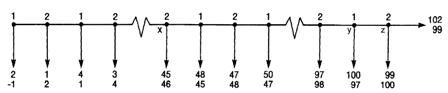
Figure 20

For the centipede, backward induction therefore recommends player 1 to play down at the first node; all other recommendations are counterfactual in the sense that no rational player should ever reach it. So what should player 2 do if he found himself at node x? Backward induction tells him to play “down’, but backward induction also told him that if player 1 was rational, he would never face the actual choice at node x. So either player 1 is rational, but made a mistake (‘trembled” in Selten’s terminology) at each node preceding x, or player 1 is not rational (Binmore 1987). But if player 1 is not rational, then player 2 may hope that she will not choose down at her next choice either, thus allowing for a later terminal node to be reached. This consideration becomes problematic for backward induction if it also affects the counterfactual reasoning. It may be the case that the truth of the indicative conditional “If player 2 finds herself at x, then player 2 is not rational” influences the truth of the counterfactual “If player 2 found herself at x, then player 2 would not be rational”. Remember that for backward induction to work, the players have to consider counterfactuals like this: “If player 2 found herself at x, and she was rational, she would choose down”. Now the truth of the first counterfactual makes false the antecedent condition of the second: it can never be true that player 2 found herself at x and be rational. Thus it seems that by engaging in these sorts of counterfactual considerations, the backward induction conclusion becomes conceptually impossible.

This is an intensely discussed problem in game theory and philosophy. Here only two possible solutions can be sketched. The first answer insists that common knowledge of rationality implies backward induction in games of perfect information (Aumann 1996). This position is correct in that it denies the connection between the indicative and the counterfactual conditional. Players have common knowledge of rationality, and they are not going to lose it regardless of the counterfactual considerations they engage in. Only if common knowledge was not immune against evidence, but would be revised in the light of the opponents’ moves, then this sufficient condition for backward induction may run into the conceptual problem sketched above. But common knowledge by definition is not revisable, so the argument instead has to assume common belief of rationality. If one looks more closely at the versions of the above argument (e.g. Pettit and Sugden (1989)), it becomes clear that they employ the notion of common belief, and not of common knowledge.

Another solution of the above problem obtains when one shows, as Bicchieri (1993, chapter 4) does, that limited knowledge of rationality and of the structure of the game suffice for backward induction. All that is needed is that a player, at each of her information sets, knows what the next player to move knows. This condition does not get entangled in internal inconsistency, and backward induction is justifiable without conceptual problems. Further, and in agreement with the above argument, she also shows that in a large majority of cases, this limited knowledge of rationality condition is also necessary for backward induction. If her argument is correct, those arguments that support the backward induction concept on the basis of common knowledge of rationality start with a flawed hypothesis, and need to be reconsidered.

In this section, I have discussed a number of possible justifications for some of the dominant game theoretic solution concepts. Note that there are many more solution concepts that I have not mentioned at all (most of them based on the Nash concept). Note also that this is a very active field of research, with new justifications and new criticisms developed constantly. All I tried to do in this section was to give a feel for some of the major problems of justification that game theoretic solution concepts encounter.

e. Paradoxes of Rationality

In the preceding section, the focus was on the justification of solution concepts. In this section, I discuss some problematic results that obtain when applying these concepts to specific games. In particular, I show that the solutions of two important games disagree with some relevant normative intuitions. Note that in both cases these intuitions go against results accepted in mainstream game theory; many game theorists, therefore, will categorically deny that there is any paradox here at all. From a philosophical point of view (as well as from some of the other social sciences) these intuitions seem much more plausible and therefore merit discussion.

The Chain Store Paradox

Recall the story from section 1c: a chain store faces a sequence of possible small-business entrants in its monopolistic market. In each period, one potential entrant can choose to enter the market or to stay out. If he has entered the market, the chain store can choose to fight or to share the market with him. Fighting means engaging in predatory pricing, which will drive the small-business entrant out of the market, but will incur a loss (the difference between oligopolistic and predatory prices) for the chain store. Thus fighting is a weakly dominated strategy for the chain store, and its threat to fight the entrant is not credible.

Because there will only be a finite number of potential entrants, the sequential game will also be finite. When the chain store is faced with the last entrant, it will cooperate, knowing that there is no further entrant to be deterred. Since the structure of the game and the chain store’s rationality are common knowledge, the last small-business will decide to enter. But since the last entrant cannot be deterred, it would be irrational for the chain store to fight the penultimate potential entrant. Thus, by backward induction, the chain store will always cooperate and the small-businesses will always decide to enter.

Selten (1978), who developed this example, concedes that backward induction may be a theoretically correct solution concept. However, for the chain-store example, and a whole class of similar games, Selten construes backward induction as an inadequate guide for practical deliberation. Instead, he suggests that the chain store may accept the backward induction argument for the last x periods, but not for the time up to x. Then, following what Selten calls a deterrence theory, the chain store responds aggressively to entries before x, and cooperatively after that. He justifies this theory (which, after all, violates the backward induction argument, and possibly the dominance argument) by intuitions about the results:

…the deterrence theory is much more convincing. If I had to play a game in the role of [the chain store], I would follow the deterrence theory. I would be very surprised if it failed to work. From my discussion with friends and colleagues, I get the impression that most people share this inclination. In fact, up to now I met nobody who said that he would behave according to the [backwards] induction theory. My experience suggests that mathematically trained persons recognize the logical validity of the induction argument, but they refuse to accept it as a guide to practical behavior. (Selten 1978, 132-3)

Various attempts have been made to explain the intuitive result of the deterrence theory on the basis of standard game theory. Most of these attempts are based on games of incomplete information, allowing the chain store to exploit the entrants’ uncertainty about its real payoffs. Another approach altogether takes the intuitive results of the deterrence theory and argues that standard game should be sensitive to limitations of the players’ rationality. Some of these limitations are discussed under the heading of bounded rationality in Section 2f.

The One-Shot Prisoners’ Dilemma

The prisoners’ dilemma has attracted much attention, because all standard game theoretic solution concepts unanimously advise each player to choose a strategy that will result in a Pareto-dominated outcome.

	C1	C2
R1	2,2	0,3
R2	3,0	1,1

Figure 21: Prisoners’ Dilemma

Recall that the unique Nash equilibrium, as well as the dominant strategies, in the prisoners’ dilemma game is (R2,C2) – even though (R1,C1) yields a higher outcome for each player. In Section 1b, the case of an infinitely repeated prisoners’ dilemma yielded a different result. Finite repetitions, however, still yield the result (R2,C2) from backward induction. That case is structurally very similar to the chain store paradox, whose implausibility was discussed above. But beyond the arguments for (R1,C1) derived from these situations, many also find the one-shot prisoners’ dilemma result implausible, and seek a justification for the players to play (R1,C1) even in that case. Gauthier (1986) has offered such a justification based on the concept of constrained maximization. In Gauthier’s view, constrained maximization bridges the gap between rational choice and morality by making moral constraints rational. As a consequence, morality is not to be seen as a separate sphere of human life but as an essential part of maximization.

Gauthier envisions a world in which there are two types of players: constrained maximizers (CM) and straightforward maximizers (SM). An SM player plays according to standard solution concepts; A CM player commits herself to choose R1 or C1 whenever she is reasonably sure she is playing with another CM player, and chooses to defect otherwise. CM players thus do not make an unconditional choice to play the dominated strategy; rather, they are committed to play cooperatively when faced with other cooperators, who are equally committed not to exploit one another’s good will. The problem for CM players is how to verify this condition. In particular in one-shot games, how can they be reasonably sure that their opponent is also CM, and thus also committed to not exploit? And how can one be sure that opponents of type CM correctly identify oneself as a CM type? With regards to these questions, Gauthier offers two scenarios, which try to justify a choice to become a CM. In the case of transparency, players’ types are common knowledge. This is indeed a sufficient condition for becoming CM, but the epistemic assumption itself is obviously not well justified, particularly in one-shot games – it simply “assumes away” the problem. In the case of translucency, players only have beliefs about their mutual types. Players’ choices to become CM will then depend on three distinct beliefs. First, they need to believe that there are at least some CMs in the population. Second, they need to believe that players have a good capacity to spot CMs, and third that they have a good capacity to spot SMs. If most players are optimistic about these latter two beliefs, they will all choose CM, thus boosting the number of CMs, making it more likely that CMs spot each other. Hence they will find their beliefs corroborated. If most players are pessimistic about these beliefs, they will all choose SM and find their beliefs corroborated. Gauthier, however, does not provide a good argument of why players should be optimistic; so it remains a question whether CM can be justified on rationality considerations alone.

f. Bounded Rationality in Game Players

Bounded rationality is a vast field with very tentative delineations. The fundamental idea is that the rationality which mainstream cognitive models propose is in some way inappropriate. Depending on whether rationality is judged inappropriate for the task of rational advice or for predictive purposes, two approaches can be distinguished. Bounded rationality which retains a normative aspect appeals to some version of the “ought implies can” principle: people cannot be required to satisfy certain conditions if in principle they are not capable to do so. For game theory, questions of this kind concern computational capacity and the complexity-optimality trade-off. Bounded rationality with predictive purposes, on the other hand, provides models that purport to be better descriptions of how people actually reason, including ways of reasoning that are clearly suboptimal and mistaken (for an overview of bounded rationality, see Grüne-Yanoff 2007). The discussion here will be restricted to the normative bounded rationality.

The outmost bound of rationality is computational impossibility. Binmore (1987) discusses this topic by casting both players in a two-player game as Turing machines. A Turing machine is a theoretical model that allows for specifying the notion of computability. Very roughly, if a Turing machine receives an input, performs a finite number of computational steps (which may be very large), and gives an output then the problem is computable. If a Turing machine is caught in an infinite regress while computing a problem, however, then the problem is not computable. The question Binmore discusses is whether Turing machines can play and solve games. The scenario is that the input received by one machine is the description of another machine (and vice versa), and the output of both machines determines the players’ actions. Binmore shows that a Turing machine cannot predict its opponent’s behavior perfectly and simultaneously participate in the action of the game. Roughly put, when machine 1 first calculates the output of machine 2 and then takes the best response to its action, and machine 2 simultaneously calculates the output of machine 1 and then takes the best response to its action, the calculations of both machines enter an infinite regress. Perfect rationality, understood as the solution to the outguessing attempt in “I thank that you think that I think…” is not computable in this sense.

Computational impossibility, however, is very far removed from the realities of rational deliberation. Take for example the way people play chess. Zermelo (1913) long ago showed that chess has a solution. Despite this result, chess players cannot calculate the solution of the game and choose their strategies accordingly. Instead, it seems that they typically “check out” several likely scenarios and that they entertain some method to evaluate the endpoint of each scenario (e.g. by counting the chess pieces). People differ in the depth of their inquiry, the quality of the “typical scenarios” selected, and the way they evaluate their endpoint positions.

The justification for such “piecemeal” deliberation is that computing the solution of a game can be very costly. Deliberation costs reduce the value of an outcome; it may therefore be rational to trade the potential gains from a full-blown solution with the moderate gains from “fast and frugal” deliberation procedures that are less costly (the term “fast and frugal” heuristics was coined by the ABC research group. Compare Gigerenzer et al 1999). Rubinstein (1998) formalizes this idea by extending the analysis of a repeated game to include players’ sensitivity to the complexity of their strategies. He restricts the set of strategies to those that can be executed by finite machines. He then defines the complexity of a strategy as the number of states of the machine that implements it. Each player’s preferences over strategy profiles increase with her payoff in the repeated game, and decrease with the complexity of her strategy’s complexity (He considers different ranking methods, in particular unanimity and lexicographic preferences). Rubinstein shows that the set of equilibria for complexity-sensitive games is much smaller than that of the regular repeated game.

3. Game Theory as a Predictive Theory

We now turn from the use of game theory as a normative theory to its use as a scientific theory of human behavior. Game theory, as part of Rational Choice Theory, is an important social scientific method. There is, however, considerable controversy about the usefulness of Rational Choice Theory for the purposes of the social sciences. Some of this controversy arises along disciplinary boundaries: while Rational Choice Theory is considered mainstream in economics (to the extent that no one even bothers using this label), sociologists and political scientists are more divided. A long debate in those disciplines reached its peak with the publications of Green and Shapiro’s (1994) Pathologies of Rational Choice Theory. In this book, they make two major claims about the scientific usefulness of Rational Choice Theory. First, they argue that Rational Choice Theory is empirically empty: that it has produced virtually no new propositions about politics that have been carefully tested and not found wanting. Second, they argue that the perceived universality claim of Rational Choice Theory is misguided: that even if an empirically successful Rational Choice Theory were to emerge, it would not be any more universal than the middle-level theories that they advocate.

These two claims have been challenged on various fronts. First, it has been pointed out that Green and Shapiro employ inappropriate standards for testing Rational Choice Theory, standards that not even successful theories of the hard sciences would survive (Diermeier 1995). Second, defenders of Rational Choice Theory have argued that Green and Shapiro’s argument relies on a biased selection of rational choice literature to survey; and further, that even in the literature they selected, there are interesting and empirically confirmed propositions that satisfy their minimum requirements (Cox 1999). Third, one can argue that Green and Shapiro’s criticism of Rational Choice Theory as a universal theory goes amiss. In Section 1c, I argued that game theory is in fact not a universal theory of rationality, but rather offers a menu of tools to model specific situations. At least with respect to game theory, therefore, they attack the wrong target: game theory is useful because it is a widely applicable method, which works well in certain circumstances, rather than a universal substantive theory of human behavior.

Although game theory cannot be dismissed as not useful for prediction just because it is part of Rational Choice Theory, game theory has a number of problems of its own that need to be discussed in depth. The first issue is to what extent the role of game theory as a theory of rationality is relevant here. I contrast this possibility with a brief sketch of evolutionary game theory, which abandons the rationality notion altogether. In the consecutive section, I discuss the problems of specifying the payoffs in a game, and thus giving a game model empirical content. Last, I discuss the possibility whether game theory can be tested at all, and investigate a recent claim that indeed game theory has been tested, and refuted.

Game theory may be useful in predicting human behavior for two distinct reasons. First, it may be the case that game theory is a good theory of rationality, that agents are rational and that therefore game theory predicts their behavior well. If game theory was correct for this reason, it could reap the additional benefit of great stability. Many social theories are inherently unstable, because agents adjust their behavior in the light of its predictions. If game theory were a good predictive theory because it was a good theory of rationality, this would be because each player expected every other player to follow the theory’s prescriptions and had no incentive to deviate from the recommended course of action. Thus, game theory would already take into account that players’ knowledge of the theory has a causal effect on the actions it predicts (Bicchieri 1993, chapter 4.4). Such a self-fulfilling theory would be more stable than a theory that predicts irrational behavior. Players who know that their opponents will behave irrationally (because a theory tells them) can improve their results by deviating from what the theory predicts, while players who know that their opponents will behave rationally cannot. However, the prospects for game theory as a theory where prescription and prediction coincide are not very good; evidence from laboratory experiments, as well as from casual observations, often puts doubt on it.

Second, and independently of the question of whether game theory is a good theory of rationality, game theory may be a good theory because it offers the relevant tools to systematize and predict interactive behavior successfully. This distinction may make sense when separating our intuitions about how agents behave rationally from a systematic account of our observations of how agents behave. Aumann for example suggests that

philosophical analysis of the definition [of Nash equilibrium] itself leads to difficulties, and it has its share of counterintuitive examples. On the other hand, it is conceptually simple and attractive, and mathematically easy to work with. As a result, it has led to many important insights in the applications, and has illuminated and established relations between many different aspects of interactive decision situations. It is these applications and insights that lend it validity. (Aumann 1985, 49).

These considerations can lead one to accept the view that the principles of game theory provide an approximate model of human deliberation, which sometimes provides insights into real phenomena (this seems to be Aumann’s position). Philosophy of Science discusses various ways of how approximate models can relate to real phenomena; each has its specific problems, which cannot be discussed here.

Aumann’s considerations can also lead one to seek an alternative interpretation of the Nash concept that does not refer to human rationality, but retains all the formally attractive properties. Evolutive approaches of game theory offer such an interpretation (Binmore 1987 proposed this term in order to distinguish it from the eductive approaches discussed in Section 2). Its proponents claim that the economic, social and biological evolutionary pressure directs human agents, who have no clear idea what is going on, to behavior that is in accord with the solution concepts of game theory.

a. The Evolutive Interpretation

The evolutive interpretation seeks to apply techniques, results, and justifications of assumptions from evolutionary game theory to game theory as a predictive theory of human behavior. Evolutionary game theory was developed in biology; it studies the appearance, robustness and stability of behavioral traits in animal populations. This article cannot do justice even to the basics of this very vibrant and expanding field (for a concise and formal introduction, see Maynard Smith 1982 and Weibull 1995), but instead presents only some aspects relevant to two questions; namely (i), to what extend can standard game theory elements be based on evolutionary game theory? And (ii), does this reinterpretation help in the prediction of human behavior?

Evolutionary game theory studies games that are played over and over again by players drawn from a populations. These players do not have a choice between strategies, but rather are “programmed” to play only one strategy. It is thus often said that the strategies themselves are the players. Success of a strategy is defined in terms of the number of replications that a strategy will leave of itself to play in games of future generations. Rather than determining equilibrium as the consequence of strategic reasoning by rational players, evolutionary game theory determines the stability of a strategy distribution in a population either as the resistance to mutant invasions, or as the result of a dynamic process of natural selection. Its equilibrium concept is thus much closer to the stable state concept of the natural sciences, where different causal factors balance each other out, than the eductive interpretation is.

Evolutionary game theory can be distinguished into a static and into a dynamic approach. The static approach specifies strategies that are evolutionary stable against a mutant invasion. Imagine a population of players programmed to play one (mixed or pure) strategy A. Imagine further that a small fraction of players “mutate” – they now play a strategy B different from A. A strategy is an evolutionary stable strategy (ESS) if for every possible mutant strategy B different from A, the payoff of playing A against the A is higher than the payoff of playing B against A – or, if both payoffs are equal, then the payoff of playing A against B is higher than playing B against B. Note that ESS is a robustness test only against a single mutation at a time. It is assumed that the population that plays an ESS has time to adjust back to status quo before the next mutant invasion begins. It follows from this definition that every ESS is a strategy that is in Nash equilibrium with itself. However, not every strategy that is Nash equilibrium with itself is an ESS.

The dynamic approach of evolutionary game theory considers a selection mechanism that favors some strategies over others in a continuously evolving population. Imagine a population whose members are programmed to play different strategies. Pairs of players are drawn at random to play against each other. Their payoff consists in an increase or decrease in fitness, measured as the number of offspring per time unit. Each offspring inherits the parent’s strategy. Reproduction takes place continuously over time, with the birthrate depending on fitness, and the death rate being uniform for all players. Long continuations of tournaments between players then may lead to stable states in the population, depending on the initial population distribution. This notion of dynamic stability is wider than that of evolutionary stability: while all evolutionary stable strategies are also dynamically stable, not all dynamically stable strategies are evolutionary stable. It has been shown that in the long run, all strictly dominated and all iteratively strictly dominated strategies are eliminated from the population. The relation between stable states and Nash equilibria is more complex, and would require specifications that go beyond the scope of this brief sketch.

Evolutionary game theory provides interesting concepts and techniques that are quite compatible with the solution concepts of standard game theory discussed in Section 1 (however, it focuses mainly on two-person static games; dynamic games and game repetitions are less investigated). Clearly, evolutionary game theory is more concerned with discovering conditions of stability and robustness of strategies in populations, than with finding the equilibria of a single game. The question that remains is whether it competes in its explanatory efforts with eductive game theory, or whether it deals instead with different (although maybe related) phenomena.

Those who claim that explanatory efforts between these two interpretations do compete hope that evolutionary concepts will replace players’ rationality – better even, that they will explain why we sometimes think that players are rational. This hope is well illustrated at the hand of Binmore’s evolutive model and the criticism directed against it. Binmore’s approach starts with the concept of a meme – “a norm, an idea, a rule of thumb, a code of conduct – something that can be replicated from one head to another by imitation or education, and that determines some aspects of the behavior of the person in whose head it is lodged” (Binmore 1994, 20). Players are mere hosts to these memes, and their behavior is partly determined by them. Fitness is a property of the meme and its capacity to replicate itself to other players. Expected utility maximization is then interpreted as a result of evolutionary selection:

People who are inconsistent [in their preferences] will necessarily be sometimes wrong and hence will be at a disadvantage compared to those who are always right. And evolution is not kind to memes that inhibit their own replication. (Binmore 1994, 27)

This is of course a version of the dynamic approach discussed above. To that extent, the theory of the fittest memes becoming relatively more frequent is an analytic truth, as long as “fitness” is no more than high “rate of replication”. But Binmore then transfers the concept of strategy fitness to player rationality. Critics have claimed that this theory of meme fitness cannot serve as the basis for the claim that the behavior of human individuals as hosts of memes will tend towards a rational pattern. The error occurs, Sugden (2001) argues, when Binmore moves from memes fitness to fitness of players. In the analogous biological case – which is based on genes instead of memes – the reproductive success of phenotype depends on the combination of genes that carry it. Genes have positive consequences in combination with some genes while bad consequences in combination with others. A gene pool in equilibrium therefore may contain genes which, when brought together in the same individual by a random process of sexual reproduction, have bad consequences for that individual’s survival and reproduction. Therefore, genes may be subject to natural selection, but there may be a stable proportion of unfit phenotypes produced by them in the population. It is thus not necessarily the case that natural selection favors phenotype survival and reproduction. The same argument holds for memes: unless it is assumed that an agent’s behavior is determined by one meme alone, natural selection on the level of memes does not guarantee that agents’ behavioral patterns are rational in the sense that they are consistent with expected utility theory. It therefore remains an empirical question whether people behave in accord with the principles game theory proposes. The evolutive interpretation cannot determine a priori that players will play Nash equilibrium.

b. The Problem of Alternative Descriptions

While intuitions about rational behavior may be teased out in fictional, illustrative stories, the question of whether prediction is successful is answerable only on the basis of people’s observed behavior. Behavioral game theory observes how people behave in experiments in which their information and incentives are carefully controlled. With the help of these experiments, and drawing on further evidence from psychology, it hopes to test game-theoretic principles for their correctness in predicting behavior. Further, in cases where the tests do not yield positive results, it hopes that the experiments suggest alternative principles that can be included in the theory (for more details on Behavioral Game Theory, their experimental methods and results, see Camerer 2003). To test game theory, the theory must be made to predict particular behavior. To construct specific experimental setups, and to make the theory predict such particular behavior, however, particular interactive phenomena need to be modeled as games, so that the theory’s solution concepts can be applied. This brings with it the problem of interpretation discussed in Section 1c. The most contentious aspect of a game modeling lies in the payoffs. The exemplary case is the disagreement over the relevant evaluations of the players in the Prisoners’ Dilemma.

Some critics of the defect/defect Nash equilibrium solution have claimed that players would cooperate because they would not only follow their selfish interests, but also take into account non-selfish considerations. They may cooperate, for example, because they care about the welfare of their opponents, because they want to keep their promises out of feelings of group solidarity or because they would otherwise suffer the pangs of a bad conscience. To bring up these considerations against the prisoners’ dilemma, however, would expose a grave misunderstanding of the theory. A proper game uses the players’ evaluation, captured in the utility function, of the possible outcomes, not the material payoff (like e.g. money). The evaluated outcome must be described with those properties the players find relevant. Thus either the non-selfish considerations are already included in the players’ payoffs (altruistic agents, after all, also have opposing interest – e.g. which charitable cause to benefit); or the players will not be playing the Prisoners’ Dilemma. They will be playing some other game with different payoffs.

Incorporating non-material interests in the payoffs has been criticized for making game theory empirically empty. The critics argue that with such a broad interpretation of the payoffs, any anomaly in the prediction of the theory can be dissolved by a re-interpretation of the agents’ evaluations of the consequences. Without constraints on re-interpretation, the critics claim, the theory cannot be held to any prediction.

To counter this objection, many economists and some game theorists claim to work on the basis of the revealed preference approach. At a minimum, this approach requires that the preferences – and hence the utility function – of an agent are exclusively inferred from that agent’s choices (for a discussion of the revealed preference account, see Grüne 2004). This ostensibly relieves game modelers to engage in “psychologizing” when trying to determine the players’ subjective evaluations.

However, it has been argued that the application of the revealed preference concept either trivializes game theory or makes it conceptually inconsistent. The first argument is that the revealed preference approach completely neglects the importance of beliefs in game theory. An equilibrium depends on the players’ payoffs and on their beliefs of what the other players believe and what they will do. In the stag hunt game of figure 1, for example, Row believes that if Col believed that Row would play R2, then he would play C2. But if the payoff numbers represented revealed preferences, Hausman (2000) argues, then they would say how individuals would choose, given what the other chose, period. The payoffs would already incorporate the influence of belief, and belief would play no further role. Game theory as a theory of rational deliberation would have lost its job.

The second criticism claims that it is conceptually impossible that games can be constructed on the basis of revealed preferences. Take as an example the simple game in figure 22.

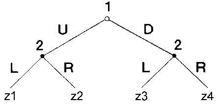
Figure 22: A game tree

How can a modeler determine the payoff pairs z1-z4 for both players according to the revealed preference method? Let’s start with player 2. Could one construct two choice situations for player 2 in which he chooses between z1 and z2 and between z3 and z4 respectively? No, argues Hausman (2000): two thus constructed choice situation exactly differ from the game in figure 22 in that they are not preceded by player 1’s choice. Hence there is no reason why it could not be the case that player 2 chooses z1 over z2 in the game but chooses z2 over z1 in the constructed choice situation. More problematically still, player 2 must be able to compare z1 with z3 and z2 with z4. But it is logically impossible that she will ever face such a choice, as player 1 will choose either U or D. Last, turning to player 1, she never faces a choice between the outcomes of this game, only between U and D. So the revealed preference theorist cannot assign preferences over outcomes to player 1 at all, and to player 2 only partially. With the preferences that he can assign – to player 2’s played strategy, and to player 1’s choices – prediction is only possible at the pain of trivializing game theory. The only prediction that the revealed preference theorist now can offer is that the players play whatever action they revealed prefer – that is, they do what they do.

These problems may have contributed to a widespread neglect of the problem of preference ascription in game theoretic models. As Weibull (2002) observes:

While experimentalists usually make efforts to carefully specify to the subject the game form … they usually do not make much effort to find the subject’s preferences, despite the fact that these preferences constitute an integral part of the very definition of a game. Instead, it is customary to simply hypothesize subjects’ preferences. (Weibull 2002, 2)

The problem of preference identification has been insufficiently addressed in rational choice theory in general and in game theory in particular. But it is not unsolvable. One solution is to find a criterion for outcome individuation. Broome offers such a criterion by justifiers: “outcomes should be distinguished as different if and only if they differ in a way that makes it rational to have a preference between them” (Broome 1991, 103). This criterion, however, requires a concept of rationality independent of the principles of rational choice. A rational choice is no longer based on preferences alone, but preferences themselves are now based on the rationality concept. This constitutes a radical departure of how most rational choice theorists, including game theorists, regard the concept of rationality. Another option that Hausman (2005) suggests is that economists can use game theoretic anomalies to study the factors influencing preferences. By altering features of the game forms and, in particular, by manipulating the precise beliefs each player has about the game and about others’ conjectures, experimenters may be able to make progress in understanding what governs choices in strategic situations and hence what games people are playing.

c. Testing Game Theory

Whether game theory can be tested depends on whether the theory makes any empirical claims, and whether it can be immunized against predictive failure.

Does the theory make testable claims? At first, it does not seem so. The theory as discussed in Sections 1a-1b mainly takes the form of theorems. Theorems are deductive conclusions from initial assumptions. So to test game theory, these assumptions need to be tested for their empirical adequacy. In this vein, Hausman (2005) claims that game theory is committed to contingent and testable axioms concerning human rationality, preferences, and beliefs. This claim remains controversial. Many economists believe that theories should not be tested with regard to their assumptions, but only with respect to their predictions (a widespread view that was eloquently expressed by Friedman 1953). But the theory only makes empirical claims in conjunction with its game models.

Further, testing game theory through its predictions is difficult as such tests must operate through the mediation of models that represent an interactive situation. Here the issue of interpreting the modeled situation (see Section 1c) and of model construction drives a wedge between the predicting theory and the real world phenomena, so that predictive failures can often be attributed to model misspecification (as discussed in section 3b).

Guala (2005) recently pointed to a specific element of game theory that seems to make an empirical claim all by itself, and independent of auxiliary hypotheses. For this purpose, he discusses the phenomenon of reciprocity. Agents reciprocate to other agents who have exhibited “trust” in them because they want to be kind to them. Reciprocation of an agent 1 to another agent 2 is necessarily dependent on 2 having performed an action that led 1 to reciprocate. Reciprocation is thus clearly delineated from general altruism or justice considerations.

The question that Guala raises is whether reciprocity can be accounted for in the payoff matrix of a game. The ‘kindness’ of an action depends on what could have been chosen: I think that you are kind to me because you could have harmed me for your benefit, but you elected not to. This would mean that the history of chosen strategies would endogenously modify the payoffs, a modeling move that is explicitly ruled out in standard game theory. Guala shows that the exclusion of reciprocity is connected right to the core of game theory: to the construction of the expected utility function. All existing versions of the existence proof of expected utility theory rely on the so-called rectangular field assumption. It assumes that decision makers form preferences over every act that can possibly be constructed by combining consequences with states of the world. However, if reciprocity has to be modeled in the consequences, and reciprocity depends on others’ acts that in turn depend on the players’ own acts, then it is conceptually impossible to construct acts in accord with the rectangular field assumption, because the act under question would be caught in an infinite regress.

If Guala’s argument is correct, it seems impossible to model reciprocity in the payoffs, and game theory is not flexible enough to accommodate reciprocity considerations into its framework. But that would mean that game theory claims that reciprocity does not exist in general. With this claim, game theory would be testable, and – if reciprocity were indeed a relevant factor in strategic decisions, as the evidence seems to suggest – would be refuted.

4. Conclusion

Game theory, this survey showed, does not provide a general and unified theory of interactive rationality; nor does it provide a positive theory of interactive behavior that can easily be tested. These observations have many implications of great philosophical interest, some of which were discussed here. Many of the questions that arise in these discussions are still left unanswered, and therefore require more attention from philosophers than they currently receive.

This article could only sketch the basic concepts of game theory in order to discuss some of their philosophical implications and problems. Wherever possible, it abstained from presenting any formal detail. To fully understand game theory, however, a formal treatment is inevitable. A good and fun introduction that also points out some philosophical issues is Binmore (1991). A textbook that puts more emphasis on the mathematical proofs is Osborne and Rubinstein (1994); a thorough and technical treatment (including excellent bibliographies) is Fudenberg and Tirole (1991). Some of the graphs found in this article were taken from that book.”

See also the discussions of game theory in these articles: Law and Economics, Egoism, Libertarianism, and Social Contract Theory.

5. References and Further Reading

Aumann, Robert. “What is Game Theory Trying to Accomplish?” Frontiers of Economics. Ed. K Arrow and S. Honkapojah. Oxford: Blackwell, 1985.
Aumann, Robert. “Backward Induction and Common Knowledge of Rationality,” Games and Economic Behavior 8 (1995): 6-19.
Bacharach, Michael. “Variable Universe Games,” Frontiers of Game Theory. Ed. Binmore, Kirman and Tani. Cambridge, Mass.: MIT Press, 1993. 255-75.
Brandenburger, Adam. “Knowledge and Equilibrium in Games,” Journal of Economic Perspectives 6 (1992): 83-101.
Bernheim, D. “Rationalizable Strategic Behavior,” Econometrica 52(1984): 1007-1028.
Bicchieri, Christina. Rationality and Coordination. Cambridge: Cambridge University Press, 1993.
Binmore, Ken. “Modeling Rational Players: Part I,” Economics and Philosophy 3 (1987): 179-214.
Binmore, Ken Fun and Games, D.C. Heath, 1991.
Binmore, Ken. Game Theory and the Social Contract. Volume I: Just Playing. Cambridge, Mass.: MIT Press, 1994.
Broome, John. Weighting Goods. Oxford: Oxford University Press, 1991. Camerer, Colin F. Behavioral Game Theory. Princeton NJ: Princeton University Press, 2003.
Cox, Gary W. “The Empirical Content of Rational Choice Theory: A Reply to Green and Shapiro,” Journal of Theoretical Politics 11(1999): 147-166.
Diermeier, Daniel “Rational Choice and the Role of Theory in political Science,” Critical Review 9 (1995): 59-70.
Ellsberg, Daniel. “Theory of the Reluctant Duelist,” The American Economic Review 46/5 (1956): 909-923.
Friedman, Milton. “The methodology of positive economics,” in Essays in Positive Economics. Chicago: University of Chicago Press, 1953, pp. 3-43.
Fudenberg, Kreps and Levine. “On the Robustness of Equilibrium Refinements,” Journal of Economic Theory 44 (1988): 354-380.
Fudenberg and Maskin. “The Folk Theorem with Discounting and with Incomplete Information,” Econometrica 54 (1986): 533-554.
Fudenberg, Drew and Jean Tirole. Game Theory. Cambridge, Mass.: MIT Press, 1991.
Gauthier, David. Morals by Agreement. Oxford: Clarendon Press, 1986
Gigerenzer, G., Todd, P. & the ABC Research Group (1999). Simple heuristics that make us smart. New York: Oxford University Press..
Goeree Jacob K. and Charles A. Holt “Ten Little Treasures of Game Theory and Ten Intuitive Contradictions,” American Economic Review 91/5 (2001): 1402-1422.
Green, Donald and Ian Shapiro. Pathologies of Rational Choice Theory, New Haven, CT: Yale University Press, 1994.
Grüne, Till. “The Problems of Testing Preference Axioms on the Basis of Revealed Preference Theory,” Analyse und Kritik 26/2 (2004): 382-397.
Grüne-Yanoff, Till “Bounded Rationality,” Philosophy Compass, Basil Blackwell, Vol. 2 (3): 534-563, 2007.
Grüne-Yanoff, Till and Sven Ove Hansson “Preferences,” The Stanford Encyclopedia of Philosophy, Edward N. Zalta (ed.), http://plato.stanford.edu/entries/preferences/, 2006.
Grüne-Yanoff, Till and Paul Schweinzer “The Role of Stories in Applying Game Theory,” Journal of Economic Methodology, 2008.
Guala, Francesco (2006) “Has Game Theory Been Refuted?” The Journal of Philosophy 103 (55): 239-263.
Hausman, Danniel M. “Revealed Preferences, Belief and Game Theory,” Economics and Philosophy 16 (2000): 99-115.
Hausman, Daniel M. “’Testing’ Game Theory,” Journal of Economic Methodology 12:2 (2005): 211-223.
Jacobsen, Hans Jørgen. “On the Foundations of Nash Equilibrium,” Economics and Philosophy 12 (1996): 67-88.
Kalai, Ehud and Ehud Lehrer. “Rational Learning Leads to Nash Equilibrium,” Econometrica 61/5 (1993): 1019-1045.
Kuhn, Harold W. “Extensive Games and the Problem of Information,” Contributions to the Theory of Games. Ed. Harold W. Kuhn and A. W. Tucker. Princeton, N.J.: Princeton University Press, 1953.
Levi, Isaac. “Prediction, Deliberation, and Correlated Equilibrium,” The Covenant of Reason. Cambridge: Cambridge University Press, 1997: 102-117.
Luce, R. Duncan and Howard Raiffa. Games and Decisions. New York: Wiley, 1957.
Morgan, Mary. “The Curious Case of the Prisoner’s Dilemma: Model Situation? Exemplary Narrative?” Science without Laws. Ed. A. Creager, M. Norton Wise and E.
Nash, John. “Equilibrium Points in n-Person Games,” Proceedings of the National Academy of Science 36 (1950): 48-49.
von Neumann, John and Oskar Morgenstern. The Theory of Games and Economic Behavior. Princeton, N.J.: Princeton University Press, 1944.
Osborne, Martin and Ariel Rubinstein. A Course in Game Theory. Cambridge, Mass.: MIT Press, 1994.
Pearce, David G. “Rationalizable Strategic Behavior and the Problem of Perfection,” Econometrica 52/4 (1984): 1029-1050.
Pettit, Philip and Robert Sugden “The Backward Induction Paradox,’ The Journal of Philosophy 86/4 (1989): 169-182.
Risse, Matthias. “What is Rational About Nash Equilibria?” Synthese 124 (2000): 361-384.
Rubinstein, Ariel. “Comments on the Interpretation of Game Theory,” Econometrica 59/4 (1991): 909-924.
Rubinstein, Ariel Modeling Bounded Rationality, MIT Press, 1998.
Schelling, Thomas. The Strategy of Conflict. Cambridge Mass.: Harvard University Press, 1960.
Selten, Reinhard. “The Chain Store Paradox.” Theory and Decision 9/2 (1978): 127-159.
Shapley, Lloyd S. “Some Topics in Two-Person Games,” in Advances in Game Theory, M. Dresher, Lloyd S. Shapley and A. W. Tucker, eds., Princeton University Press,1-28, 1964.
Stalnaker, Robert. “Knowledge, Belief and Counterfactual Reasoning in Games,” The Logic of Strategy. Ed. C. Bicchieri, R. Jeffrey, B. Skyrms. Oxford University Press, 1999.
Sugden, Robert. “A Theory of Focal Points,” Economic Journal 105 (1995): 1296-302.
Sugden, Robert. “The Evolutionary Turn in Game Theory,” Journal of Economic Methodology 8/1 (2001): 113-130.
Weibull, Jörgen W. Evolutionary Game Theory. Cambridge, Mass.: MIT Press, 1995.
Weibull, Jörgen W. “Testing Game Theory,” Mimeo, 2004.
Young, H. Peyton. Individual Strategy and Social Strategy: An Evolutionary Theory of Institutions. Princeton, NJ: Princeton University Press, 2001.
Zermelo, Ernst. “Über eine Anwendung der Mengenlehre auf die Theorie des Schachspiels,” Proceedings of the Fifth International Congress on Mathematics, 1913.

Author Information

Till Grüne-Yanoff
Email: gruneyan@mappi.helsinki.fi
University of Helsinki
Finland

Internet Encyclopedia of Philosophy