Set Theory
Set Theory is a branch of mathematics that investigates sets and their properties. The basic concepts of set theory are fairly easy to understand and appear to be self-evident. However, despite its apparent simplicity, set theory turns out to be a very sophisticated subject. In particular, mathematicians have shown that virtually all mathematical concepts and results can be formalized within the theory of sets. This is considered to be one of the greatest achievements of modern mathematics. Given this achievement, one can claim that set theory provides a foundation for mathematics.
The foundational role of set theory and its mathematical development have raised many philosophical questions that have been debated since its inception in the late nineteenth century. For example, here are three: Does infinity exist, and if so, are there different kinds of infinity? Is there a mathematical universe? Are all mathematical problems solvable?
Before pursuing the philosophical issues concerning set theory, one should be familiar with a standard mathematical development of set theory. This article presents such a development.
In the late nineteenth century, the mathematician Georg Cantor (1845–1918) created and developed a mathematical theory of sets. This theory emerged from his proof of an important theorem in real analysis. In this proof, Cantor introduced a process for forming sets of real numbers that involved an infinite iteration of the limit operation. Cantor’s novel proof led him to a deeper investigation of sets of real numbers and to his theory of abstract sets. Cantor’s creation now pervades all of mathematics and offers a versatile tool for exploring concepts that were once considered to be ineffable, such as infinity and infinite sets.
Sections 1 and 2 below describe the “naïve” principles of set theory that were used and developed by Cantor. Then, Section 3 describes a more sophisticated (axiomatic) approach to set theory that arose from the discovery of Russell’s paradox. After identifying the Zermelo-Frankel axioms of set theory, Section 4 discusses Cantor’s well-ordering principle and examines how Cantor used the well-ordering principle to develop the ordinal and cardinal numbers. Section 5 considers controversies concerning the well-ordering principle and its equivalent, the axiom of choice. This is followed by introducing the cumulative hierarchy of sets, Kurt Gödel’s universe of constructible sets, and Paul Cohen’s method of forcing in Sections 6, 7, and 8, respectively. The latter two topics, explored in Sections 7 and 8, can be used to show that certain questions are unresolvable when assuming the Zermelo-Frankel axioms (with or without the axiom of choice). The next two sections address further developments in set theory that are intended to settle these and other unresolved questions; namely, Section 9 discusses large cardinal axioms, and Section 10 investigates the axiom of determinacy.
Table of Contents
- On the Origins
- Cantor’s Development of Set Theory
- The Zermelo-Fraenkel Axioms
- Cantor’s Well-Ordering Principle
- The Axiom of Choice
- The Cumulative Hierarchy
- Gödel’s Constructible Universe
- Cohen’s Forcing Technique
- Large Cardinal Axioms
- The Axiom of Determinacy
- Concluding Remarks
- References and Further Reading
1. On the Origins
Let us first discuss a few basic concepts of set theory. A set is a well-defined collection of objects. The items in such a collection are called the elements or members of the set. The symbol “\(\in\)” is used to indicate membership in a set. Thus, if \(A\) is a set, we write \(x \in A\) to say that “\(x\) is an element of \(A\),” or “\(x\) is in \(A\),” or “\(x\) is a member of \(A\).” We also write \(x \notin A\) to say that \(x\) is not in \(A\). In mathematics, a set is usually a collection of mathematical objects, for example, numbers, functions, or other sets.
Sometimes a set is identified by enclosing a list of its elements by curly brackets; for example, a set of natural numbers \(A\) can be identified by the notation
\(A = \{1,2,3,4,5,6,7,8,9\}\).
More typically, one forms a set by enclosing a particular expression within curly brackets, where the expression identifies the elements of the set. To illustrate this method of identifying a set, we can form a set B of even natural numbers, using the above set \(A\), as follows:
\(B = \{n \in A : n \text{ is even}\}\).
which can be read as “the set of \(n \in A\) such that \(n\) is even.” Of course,
\(\{n \in A : n\) is even\(\} = \{2,4,6,8\}\).
It is difficult to identify the genesis of the set concept. Yet, the idea of a finite collection of objects has existed for as long as the concept of counting. Indeed, mathematicians have been investigating finite sets and methods for measuring the size of finite sets since the beginning of mathematics. For example, the above two sets
\(B=\{2,4,6,8\}\)
are finite sets. As every element in \(B\) is an element in \(A\), the set \(B\) is said to be a subset of \(A\), denoted by \(B \subseteq A\). Since there are elements in \(A\) that are not in \(B\), we say that \(B\) is a proper subset of \(A\). Moreover, the number of elements in \(B\) is strictly smaller than the number of elements in \(A\). Thus, one can say, “the whole \(A\) is greater in size than its proper part \(B\).”
Infinite sets lead to an apparent contradiction. Consider the infinite sets:
\(D=\{1,3,5,7, \ldots \}\).
We view the sets \(C\) and \(D\) as existing entities that both contain infinitely many elements. Thus, \(C\) and \(D\) are “completed infinities.” Observe that every element in \(D\) is in \(C\), and that \(D\) is a proper subset of \(C\). However, if, as many mathematicians once believed, “infinity cannot be greater than infinity,” then the whole \(C\) is not greater in size than its proper part \(D\). This counterintuitive result was viewed by many early prominent mathematicians as being contradictory, as it appeared to conflict with the well-understood behavior of finite sets. These mathematicians thus concluded that the concept of a “completed infinity” should not be allowed in mathematics.
For this reason, before Cantor, a majority of mathematicians considered infinite collections to be mathematically illicit objects. Cantor was the first mathematician to view infinite sets as being legitimate mathematical objects that can coexist with finite sets. Clearly, the size of a finite set can be measured simply by counting the number of elements in the set. Cantor was the first to investigate the following question:
Can the concept of “size” be extended to infinite sets?
Cantor addressed this question in the affirmative by using the concept of a function to measure and compare the sizes of infinite sets. Functions are widely used in science and mathematics. For sets \(A\) and \(B\), we say that \(f\) is a function from \(A\) to \(B\), denoted by \(f\): \(A \rightarrow B\), if and only if \(f\) is a relation (operation) that assigns to each element \(x\) in \(A\), a single element \(f(x)\) in \(B\). There are three important properties that a function might possess:
- \(f\): \(A \rightarrow B\) is an injection if and only if for each \(y\) in \(B\) there is at most one \(x\) in \(A\) such that \(f(x)=y\).
- \(f\): \(A \rightarrow B\) is a surjection if and only if for each \(y\) in \(B\) there is at least one \(x\) in \(A\) such that \(f(x)=y\).
- \(f\): \(A \rightarrow B\) is a bijection if and only if for each \(y\) in \(B\) there is exactly one \(x\) in \(A\) such that \(f(x)=y\).
Observe that \(f\): \(A \rightarrow B\) is an injection if and only if distinct elements in \(A\) are assigned to distinct elements in \(B\); that is, for all \(x\) and \(a\) in \(A\), if \(x \neq a\), then \(f(x) \neq f(a)\). Also note that \(f\): \(A \rightarrow B\) is a bijection if and only if \(f\): \(A\rightarrow B\) is an injection and a surjection.
Cantor observed that two sets \(A\) and \(B\) have the same size if and only if there is a one-to-one correspondence between \(A\) and \(B\), that is, there is a way of evenly matching the elements in \(A\) with the elements in \(B\). In other words, Cantor noted that the sets \(A\) and \(B\) have the same size if and only if there is a bijection \(f\): \(A \rightarrow B\). In this case, Cantor said that \(A\) and \(B\) have the same cardinality. For an illustration, let \(\mathbb{N} = \{0, 1, 2, 3, 4, \ldots \}\) be the set of natural numbers and let \(E = \{0,2,4,6,8,\ldots\}\) be the set of even natural numbers. Now let \(f\): \(\mathbb{N} \rightarrow E\) be defined by \(f(n)=2n\). One can verify that \(f\): \(\mathbb{N} \rightarrow E\) is a bijection and, thus, we obtain the following one-to-one correspondence between the set \(\mathbb{N}\) of natural numbers and the set \(E\) of even natural numbers:

Hence, each natural number \(n\) corresponds to the even number \(2n\), and each even natural number \(2i\) is thereby matched with \(i \in \mathbb{N}\). The bijection \(f\): \(\mathbb{N} \rightarrow E\) specifies a one-to-one match-up between the elements in \(\mathbb{N}\) and the elements in \(E\). Cantor concluded that the sets N and E have the same cardinality.
Cantor also defined what it means for a set \(C\) to be smaller, in size, than a set \(D\). Specifically, he said that \(C\) has smaller cardinality (smaller size) than \(D\) if and only if there is an injection \(f\): \(C \rightarrow D\) but there is no bijection \(g\): \(C \rightarrow D\). Cantor then proved that there is no one-to-one correspondence between the set of real numbers and the set of natural numbers. Cantor’s proof showed that the set of real numbers has larger cardinality than the set of natural numbers (Cantor 1874). This stunning result is the basis upon which set theory became a branch of mathematics.
The natural numbers \(0, 1, 2, 3, \ldots\) are the whole numbers that are typically used for counting. The real numbers are those numbers that appear on the number line. For example, the natural number \(2\), the integer \(-3\), the fraction \(6/5\), and all of the other rational numbers are real numbers. The irrational numbers, such as \(\sqrt{2}\) and \(\pi\), are also real numbers. Again, let \(\mathbb{N} = \{0, 1, 2, 3, \ldots \}\) be the set of natural numbers, and let \(\mathbb{R}\) be the set of real numbers. If a set is either finite or has the same cardinality as the set of natural numbers, then Cantor said that it is countable. Since the set of real numbers \(\mathbb{R}\) is larger, in size, than the set of natural numbers \(\mathbb{N}\), Cantor referred to the set \(\mathbb{R}\) as being uncountable.
After proving that the set of real numbers is uncountable, Cantor was able to prove that there is an increasing sequence of larger and larger infinite sets. In other words, Cantor showed that there are “infinitely many different infinites,” a result with clear philosophical and mathematical significance.
After his introduction of uncountable sets, in 1878, Cantor announced his Continuum Hypothesis (CH), which states that every infinite set of real numbers is either the same size as the set of natural numbers or the same size as the entire set of real numbers. There is no intermediate size. Cantor struggled, without success, for most of his career to resolve the Continuum Hypothesis. The problem persisted and became one of the most important unsolved problems of the twentieth century. After Cantor’s death, most set theorists came to believe that the Continuum Hypothesis is unresolvable.
Cantor’s profound results on the theory of infinite sets were counterintuitive to many of his contemporaries. Moreover, Cantor’s set theory violated the prevailing dogma that the notion of a “completed infinity” should not be allowed in mathematics. Thus, the outcry of opposition persisted. Influential mathematicians continued to argue that Cantor’s work was subversive to the true nature of mathematics. These mathematicians believed that infinite sets were dangerous fictional creations of Cantor’s imagination and that Cantor’s fictions needed to be eradicated from mathematics (Dauben 1979, page 1) (Dunham 1990, pp. 278-280). Nevertheless, Cantor’s theory of sets soon became a crucial tool used in the discovery and establishment of new mathematical results, for example, in measure theory and the theory of functions (Kanamori 2012). Mathematicians slowly began to see the utility of set theory to traditional mathematics. Accordingly, attitudes started to change and Cantor’s ideas began to gain acceptance in the mathematical community (Dauben 1979, pp. 247-248). The significance of Cantor’s mathematical research was eventually recognized. David Hilbert, a prominent twentieth century mathematician, described Cantor’s work as being
the finest product of mathematical genius and one of the supreme achievements of purely intellectual human activity. (Hilbert 1923)
Ultimately, Cantor’s theory of abstract sets would dramatically change the course of mathematics.
2. Cantor’s Development of Set Theory
In his development of set theory, Cantor identified a single fundamental principle, called the Comprehension Principle, under which one can form a set. Cantor’s principle states that, given any specific property \(\varphi(x)\) concerning a variable \(x\), the collection \(\{x : \varphi(x)\}\) is a set, where \(\{x : \varphi(x)\}\) is the set of all objects \(x\) that satisfy the property \(\varphi(x)\). For example, let \(\psi(x)\) be the property that “\(x\) is an odd natural number.” The Comprehension Principle implies that
\(S = \{ x : \psi (x)\} = \{1,3,5,7,\ldots \}\)
is a set. Employing the Comprehension Principle, one can form the intersection of two sets \(A\) and \(B\) using the property “\(x \in A\) and \(x \in B\)”; thus, the intersection of \(A\) and \(B\) is the set
\(A \cap B = \{x : x \in A\) and \(x \in B\}\).
One can also form the set
\(A \cup B = \{x : x \in A\) or \(x \in B\}\)
which is called the union of \(A\) and \(B\). Recall that one writes \(X \subseteq A\) to mean that \(X\) is a subset of \(A\), that is, every element of \(X\) is also an element of \(A\). Using the Comprehension Principle, one can form the power set of \(A\), which is the set whose elements are all of the subsets of \(A\), that is,
\(\wp(A) = \{ X : X \subseteq A\}.\)
Thus, if \(A\) is a set and \(X \subseteq A\), then \(X \in \wp(A)\). So, if \(A = \{1,2,3\}\) and \(B = \{3,4,5\}\), then
\(\wp(A) = \{\varnothing,\{1\},\{2\},\{3\},\{1,2\},\{1,3\},\{2,3\},\{1,2,3\}\}\),
where \(\varnothing\) denotes the empty set, that is, the set that contains no elements. The Comprehension Principle was an essential tool that allowed Cantor to form many important sets. Cantor’s approach to set theory is often referred to as naïve set theory.
Cantor’s set theory soon became a very powerful tool in mathematics. In the early 1900s, the mathematicians Émile Borel, René-Loius Baire, and Henri Lebesgue used Cantor’s set theoretic concepts to develop modern measure theory and function theory (Kanamori 2012). This work clearly demonstrated the great mathematical utility of set theory.
a. Russell’s Paradox
The philosopher and mathematician Bertrand Russell was interested in Cantor’s work and, in particular, Cantor’s proof of the following theorem, which implies that the cardinality of the power set of a set is larger than the cardinality of the set. First, recall that a function \(g\): \(A \rightarrow B\) is a surjection (or is onto \(B\)) if for all \(y \in B\), there is an \(x \in A\) such that \(g(x)=y\).
Cantor’s Theorem. Let \(A\) be a set. Then there is no surjection \(f\): \(A \rightarrow \wp(A)\).
Proof. Suppose, for the sake of obtaining a contradiction, that there exists a surjection \(f\): \(A \rightarrow \wp(A)\). Observe that, for all \(z \in A\), \(f(z) \subseteq A\). By the Comprehension Principle, let \(X\) be the set
\(X = \{x : x \in A\) and \(x \notin f(x)\}\).
Clearly, \(X \subseteq A\). Thus, \(X \in \wp (A)\). As \(f\) is onto \(\wp(A)\), there is an \(a \in A\) such that \(f(a) = X\). There are two cases to consider: either \(a \in X\) or \(a \notin X\). If \(a \in X\), then the definition of \(X\) implies that \(a \notin f(a)\). Since \(f(a) = X\), we have that \(a \notin X\), which is a contradiction. On the other hand, if \(a \notin X\), then the definition of \(X\) implies that \(a \in f(a)\). Since \(f(a) = X\), we see that \(a \in X\), a contradiction. Thus, there is no surjection \(f\): \(A \rightarrow \wp(A)\). This completes the proof.
In 1901, after reading Cantor’s proof of the above theorem, that was published in 1891, Bertrand Russell discovered a devastating contradiction that follows from the Comprehension Principle. This contradiction is known as Russell’s Paradox. Consider the property “\(x \notin x\)”, where \(x\) represents an arbitrary set. By the Comprehension Principle, we conclude that
\(A = \{x : x \notin x\}\)
is a set. The set \(A\) consists of all the sets \(x\) that satisfy \(x \notin x\). Clearly, either \(A \in A\) or \(A \notin A\). Suppose \(A \in A\). Then, the definition of the set \(A\) implies that \(A\) must satisfy the property \(A \notin A\), which contradicts our supposition. Suppose \(A \notin A\). Since \(A\) satisfies \(A \notin A\), we infer, from the definition of \(A\), that \(A \in A\), which is also a contradiction.
There were similar paradoxes discovered by others, including Cantor (Dauben 1979), but Russell’s paradox is the easiest to understand. These paradoxes appeared to threaten Cantor’s fundamental principle that he used to develop set theory. Nevertheless, Cantor did not believe that these paradoxes actually refuted his development of set theory. He knew that the construction of certain collections can lead to a contradiction. Cantor referred to these collections as “inconsistent multiplicities.” Today, such collections are called proper classes, and the paradoxes can be used to prove that they are not sets.
3. The Zermelo-Fraenkel Axioms
Over time, it became clear that, to resolve the paradoxes in Cantor’s set theory, the Comprehension Principle needed to be modified. Thus, the following question needed to be addressed:
How can one correctly construct a set?
Ernst Zermelo (1871–1953) observed that to eliminate the paradoxes, the Comprehension Principle could be restricted as follows: Given any set \(A\) and any property \(\psi (x)\), one can form the set \(\{x \in A : \psi (x)\}\), that is, the collection of all elements \(x \in A\) that satisfy \(\psi (x)\), is a set. Zermelo’s approach differs from Cantor’s method of forming a set. Cantor declared that for every property one can form a set of all the objects that satisfy the property. Zermelo adopted a different approach: To form a set, one must use a property together with a set.
Zermelo also realized that in order to more fully develop Cantor’s set theory, one would need additional methods for forming sets. Moreover, these additional methods would need to avoid the paradoxes. In 1908, Zermelo published an axiomatic system for set theory that, to the best of our knowledge, avoids the difficulties faced by Cantor’s development of set theory. In 1930, after receiving some proposed revisions from Abraham Fraenkel, Zermelo presented his final axiomatization of set theory, now known as the Zermelo-Fraenkel axioms and denoted by ZF. These axioms have become the accepted formulation of Cantor’s ideas about the nature of sets.
a. The Axioms
As noted by Zermelo, to avoid paradoxes, the Comprehension Principle can be replaced with the principle: Given a set \(A\) and a property \(\varphi (x)\) with a variable \(x\), the collection \(\{x \in A : \varphi (x)\}\) is a set. However, this raises a new question: What is a property? The most favored way to address this question is to express the axioms of set theory in the formal language of first-order logic, and then declare that its formulas designate properties. This language involves variables and the logical connectives \(\wedge\) (and), \(\vee\) (or), \(\neg\) (not), → (if … then …), and ↔ (if and only if), together with the quantifier symbols \(\forall\) (for all) and \(\exists\) (there exists). In addition, this language uses the relation symbols \(=\) and \(\in\) (as well as \(\neq\) and \(\notin\)). In this language, the variables and quantifiers range over sets and only sets. A formula constructed in this formal language is referred to as a formula in the language of set theory. Such formulas are used to give meaning to the notion of “property.”
We now illustrate the expressive power of this set theoretic language. The formula \(\exists x(x \in A)\) asserts that “the set \(A\) is nonempty,” and \(\forall x(x \notin A)\) states that “\(A\) has no elements.” Moreover \(\neg \exists x \forall y(y \in x)\) states that “it is not the case that there is a set that contains all sets as elements.” In addition, one can translate English statements, which concern sets, into the language of set theory. For example, the English sentence “the set \(A\) contains at least two elements” can be translated into the language of set theory by \(\exists x \exists y((x \in A \wedge y \in A) \wedge x \neq y)\).
There is another quantifier, called the uniqueness quantifier, that is sometimes used. This quantifier is written as \(\exists ! x \varphi (x)\) and it means that “there exists a unique \(x\) satisfying \(\varphi (x)\).” This is in contrast with \(\exists x \varphi(x)\), which simply states that “at least one \(x\) satisfies \(\varphi (x)\).” The uniqueness quantifier is used as a convenience, as the assertion \(\exists !x \varphi (x)\) can be expressed in terms of the other quantifiers \(\exists\) and \(\forall\); namely, it is equivalent to the formula
\(\exists x \varphi (x) \wedge \forall x \forall y ((\varphi (x) \wedge \varphi (y)) \rightarrow x=y)\).
The above formula is equivalent to \(\exists!x \varphi (x)\) because it asserts that “there is an \(x\) such that \(\varphi(x)\) holds, and any sets \(x\) and \(y\) that satisfy \(\varphi (x)\) and \(\varphi(y)\) must be the same set.”
The Zermelo-Fraenkel axioms are listed below. Each axiom is first stated in English and then written in logical form. After each logical form, there is a discussion of the axiom and some of its consequences. When reading these axioms, keep in mind that, in Zermelo-Fraenkel set theory, everything is a set, including the elements of a set. Also, the notation \(\vartheta (x, \ldots, z)\) means that \(x, \ldots, z\) are free variables in the formula \(\vartheta\) and that \(\vartheta\) is allowed to contain parameters (free variables other than \(x, \ldots, z\)) that represent arbitrary sets.
Extensionality Axiom. Two sets are equal if and only if they have the same elements.
\(\forall A \forall B ( A = B \leftrightarrow \forall x ( x \in A \leftrightarrow x \in B))\).
The extensionality axiom is essentially a “definition” that states that two sets are equal if and only if they have exactly the same elements.
Empty Set Axiom. There is a set with no elements.
\(\exists A \forall x ( x \notin A)\).
The empty set axiom states that there is a set which has no elements. Since the extensionality axiom implies that this set is unique, we let \(\varnothing\) denote the empty set.
Subset Axiom. Let \(\varphi(x)\) be a formula. For every set \(A\), there is a set \(S\) that consists of all the elements \(x \in A\) such that \(\varphi(x)\) holds.
\(\forall A \exists S \forall x ( x \in S \leftrightarrow ( x \in A \wedge \varphi (x)))\).
(The variable \(S\) is assumed not to appear in the formula \(\varphi (x)\).) The subset axiom, also known as the axiom of separation, asserts that any definable sub-collection of a set is itself a set, that is, for any formula \(\varphi(x)\) and any set \(A\), the collection \(\{x \in A : \varphi(x)\}\) is a set. Clearly, the subset axiom is a limited form of the Comprehension Principle. Yet, it does not lead to the contradictions that result from the Comprehension Principle. The subset axiom is, in fact, an axiom schema since it yields infinitely many axioms-one for each formula \(\varphi\).
Pairing Axiom. For every \(u\) and \(v\), there is a set that consists of just \(u\) and \(v\).
\(\forall u \forall v \exists P \forall x ( x \in P \leftrightarrow ( x =u \vee x = v))\).
The pairing axiom states that, for any two sets \(u\) and \(v\), the set \(\{u, v\}\) exists. Thus, by the extensionality axiom, the set \(\{u, u\} = \{u\}\) exists.
Union Axiom. For every set \(F\), there exists a set \(U\) that consists of all the elements that belong to at least one set in \(F\).
\(\forall F \exists U \forall x ( x \in U \leftrightarrow \exists C (C \in F \wedge x \in C))\).
The union axiom states that, for any set \(F\), there is a set \(U\) whose elements are precisely those elements that belong to an element of \(F\), that is, \(x \in U\) if and only if \(x \in A\) for some \(A \in F\). The extensionality axiom implies that the set \(U\) is unique; it is often denoted by \(\bigcup F\). For example, consider the set \(\{A,B\}\). Then
\(\bigcup \{A,B\} = \{x : x\) belongs to a member of \(\{A,B\}\} = \{x : x \in A\) or \(x \in B\} = A \cup B\).
For another example, let \(F = \{ \{a,b,c\},\{e,f\},\{e,c,d\} \}\). Then \(\bigcup F = \{a,b,c,d,e,f\}\).
Power Set Axiom. For every set \(A\), there exists a set \(P\) that consists of all the sets that are subsets of \(A\).
\(\forall A \exists P \forall x ( x \in P \leftrightarrow \forall y( y \in x \rightarrow y \in A))\).
The power set axiom states that, for any set \(A\), there is a set, which we denote by \(\wp(A)\), such that for any set \(B\), \(B \in \wp(A)\) if and only if \(B \subseteq A\).
Infinity Axiom. There is a set \(I\) that contains the empty set as an element and whenever \(x \in I\), then \(x \cup \{x\} \in I\).
\(\exists I ( \varnothing \in I \wedge \forall x (x \in I \rightarrow x \cup \{ x \} \in I))\).
The infinity axiom ensures the existence of at least one infinite set. For any set \(x\), the successor of \(x\) is defined to be the set \(x^{+} = x \cup \{x\}\). Thus, the axiom of infinity asserts that there is a set \(I\) such that \(\varnothing \in I\) and if \(x \in I\), then \(x^{+} \in I\). Note that \(\varnothing^{+} = \{\varnothing\}\), and that \(\{\varnothing\}^{+} = \{\varnothing,\{\varnothing\}\}\). It follows that the set \(I\) contains each of the sets
\(\varnothing; \{\varnothing\}; \{\varnothing, \{\varnothing \}\}; \{\varnothing, \{\varnothing, \{\varnothing \}\}\}; \ldots\).
One can show that any two of the sets in the above list (separated by a semi-colon) are distinct. Hence, the set \(I\) contains an infinite number of elements; in other words, \(I\) is an infinite set. So, the infinity axiom simply states that infinite sets exist and are legitimate mathematical objects. The infinity axiom is a key tool that is used to develop the set of natural numbers \(\mathbb{N}\) and to prove that \(\mathbb{N}\) is well-ordered, that is, every nonempty set of natural numbers has a least element.
Replacement Axiom. Let \(\psi (x, y)\) be a formula. For every set \(A\), if for each \(x \in A\) there is a unique \(y\) such that \(\psi (x, y)\), then there is a set \(S\) that consists of all of the elements \(y\) such that \(\psi (x, y)\) for some \(x \in A\). (Below, \(\exists\)! is the uniqueness quantifier.)
\(\forall A (\forall x ( x \in A \rightarrow \exists ! y \psi (x,y)) \rightarrow \exists S \forall y( y \in S \leftrightarrow \exists x (x \in A \wedge \psi(x, y))))\).
(The variable \(S\) is assumed not to appear in the formula \(\psi (x, y)\).) The replacement axiom states that for every set \(A\), if for each \(x \in A\) there is a unique \(y\) such that \(\psi(x,y)\), then the collection \(\{y\) : \(\exists x (x \in A \wedge \psi(x,y))\}\) is a set; that is, a “functional image of a set, is a set.” The replacement axiom is a special form of Cantor’s Comprehension Principle that plays a critical role in modern set theory. However, the replacement axiom does not lead to the contradictions that follow from the Comprehension Principle. Like the subset axiom, the replacement axiom is an axiom schema. Accordingly, there are infinitely many Zermelo-Fraenkel axioms.
Regularity Axiom. Each nonempty set \(A\) contains an element that is disjoint from \(A\).
\(\forall A ( A \neq \varnothing \rightarrow \exists x ( x \in A \wedge \neg \exists y ( y \in x \wedge y \in A)))\).
The regularity axiom, also known as the axiom of foundation, states that, for any nonempty set \(A\), there is a set \(x \in A\) such that \(A \cap x = \varnothing\). The regularity axiom rules out the possibility of a set belonging to itself. In standard mathematics, there are no sets that are members of themselves. For example, the set of natural numbers is not a natural number. The regularity axiom eliminates collections that are not relevant for standard mathematics. The regularity and pairing axioms imply that if \(a \in b\), then \(b \notin a\). To see this, suppose that \(a \in b\). Then it follows, from regularity, that \(a \cap \{a,b\} = \varnothing\). So \(b \notin a\).
The Zermelo-Fraenkel axioms are now the most widely accepted answer to the question: How can one correctly construct a set? Of course, these axioms are more restrictive than Cantor’s Comprehension Principle; however, no one, in over 100 years, has been able to derive a contradiction from these axioms. Moreover, all of the classic results (excluding the paradoxes) that were derived using Cantor’s naïve set theory can be derived from the Zermelo-Fraenkel axioms.
It is a remarkable fact that essentially all mathematical objects can be defined as sets within Zermelo-Fraenkel set theory. For example, functions, relations, the natural numbers, and the real numbers can be defined within Zermelo-Fraenkel set theory. Hence, effectively all theorems of mathematics can be considered as statements about sets and proven from the Zermelo-Fraenkel axioms.
b. Classes
The argument used in Russell’s Paradox can be applied to prove, in ZF, that there is no set that contains all sets (as elements). As every set is equal to itself, the collection \(\{x\) : \(x = x\}\) contains every set, but this collection is not a set. Thus, given a formula \(\varphi(x)\), one cannot necessarily conclude that the collection \(\{x : \varphi(x)\}\) is a set. However, in set theory, it is convenient to be able to discuss such collections. They cannot be called sets. Instead, a collection of the form \(\{x\) : \(\varphi(x)\}\) is called a class. The collection \(\{x : x = x\}\) is a class that is not a set; for this reason, it is called a proper class.
When can one prove that a class is a set? Let us say that a class \(\{x : \varphi(x)\}\) is bounded if and only if there is a set \(A\) such that for all \(x\), if \(\varphi(x)\), then \(x \in A\). Using the subset axiom, one can prove that a bounded class is a set. It follows that the class \(\{x : x = x\}\) is not bounded.
In the Zermelo-Fraenkel axioms, there is no explicit mention of classes. However, there are alternative axiomatizations of set theory that extend ZF by including classes as objects in the language, that is, these axiom systems give classes a formal state of existence. The most common such axiomatic treatment of classes is denoted by NBG (von Neumann–Bernays–Gödel). The NBG system uses a formal language that has two different types of variables: capital letters denote classes and lowercase letters denote sets. In addition, classes can contain only sets as elements. So, a class that is not a set cannot belong to a class. Thus, a class \(X\) is a set if and only if \(\exists Y (X \in Y)\). In the NBG system, sets satisfy all of the ZF axioms, and the intersection of a class with a set is a set, that is, \(X \cap y\) is a set. The NBG system also has the class comprehension axiom:
\(\exists X \forall y (y \in X \leftrightarrow \varphi (y))\)
where the formula \(\varphi(y)\) can contain set parameters and/or class parameters (with other restrictions). Thus, the class comprehension axiom asserts that \(\{x : \varphi(x)\}\) is a class.
The NBG system is a conservative extension of ZF; that is, a sentence with only lowercase (set) variables is provable in NBG if and only if it is provable in ZF. The Zermelo-Fraenkel system has a clear advantage over NBG, namely, the simplicity of working with only one type of object (sets) rather than two types of objects (sets and classes). The Zermelo-Fraenkel axiomatic system is the standard system of axioms for modern set theory.
4. Cantor’s Well-Ordering Principle
As proposed by Cantor, two sets \(A\) and \(B\) have the same cardinality if and only if there is a bijection \(f\): \(A \rightarrow B\). When \(A\) is a finite set, there is a unique natural number, denoted by |\(A\)|, that identifies the number of elements in \(A\). In this case, we say that |\(A\)| is the cardinality of \(A\). For example, if \(A = \{3,5,7,2\}\), then |\(A\)| \(= 4\). Clearly, the cardinality of a finite set identifies the number of elements that are in the set. Moreover, if \(A\) and \(B\) are both finite sets, then one can prove that
(\(\Delta\))
With this understanding, Cantor asked the following question:
Are there values that can represent the size of infinite sets and satisfy (\(\Delta\))?
In other words, given two infinite sets \(A\) and \(B\), can one assign values |\(A\)| and |\(B\)| such that
|\(A\)| = |\(B\)| if and only if there exists a bijection \(f\): \(A \rightarrow B\)?
Cantor answered this question, in the affirmative, by developing the transfinite ordinal numbers, which are “infinite numbers” in the sense that they are larger than all of the natural numbers, and are well-ordered just like the natural numbers. Cantor believed that each infinite set can be assigned a specific ordinal number and that this ordinal number would measure the size of the set. Cantor realized that, in order to successfully apply his theory of ordinal numbers, he needed an additional principle. In 1883, he proposed the following principle.
Well-Ordering Principle: It is always possible to bring any well-defined set into the form of a well-ordered set.
A relation \(\leq\) on a set \(X\) is a well-ordering of \(X\) if and only if it is a total ordering in which every non-empty subset of \(X\) has a least element, where it is assumed that the relation \(\leq\) does not apply to any elements that are not in \(X\). If a set can be well-ordered, then one can generalize the concepts of induction and recursion, similar to mathematical induction, on the elements of the set. Given any infinite set, Cantor used the well-ordering principle to identify an ordinal number that measures the size of the set. Such an ordinal is called a cardinal number.
a. Ordinal Numbers
The natural numbers are often used for two purposes: to indicate the position of an element in a sequence and to identify the size of a finite set. In other words, a natural number can be used to identify a position (first, second, third, …) and it can be used to identify a size (one, two, three, …). Cantor extended the natural numbers by introducing the concepts of transfinite position and transfinite size. Suppose that we want to count the number of real numbers. As noted in Section 1, Cantor proved that the set of real numbers is uncountable. Thus, if we attempted to assign each real number to exactly one of the natural numbers \(0, 1, 2, 3, \ldots,\) then we would not have enough natural numbers to complete this task. However, suppose that we add some new numbers, called transfinite ordinals, to our stock of numbers. Clearly, we need an ordinal that will identify the first position that occurs after all of the natural numbers. Cantor denoted this ordinal by the Greek letter \(\omega\). That is, Cantor proposed the following “position” sequence
(1)
Observe the following:
- By starting with \(0\) and repeatedly adding \(1\), we obtain all of the natural numbers.
- Every natural number greater than \(0\) has an immediate predecessor; for example, \(5\) has \(4\) as its immediate predecessor.
By contrast, the ordinal number \(\omega\) cannot be obtained by repeatedly adding \(1\) to \(0\) and it does not have an immediate predecessor. For these reasons, we say that \(\omega\) is a limit ordinal.
We can continue the sequence (1) by repeatedly adding \(\) to \(\omega\). By doing so, we obtain the following position sequence:
(2)
The process for constructing (1) and (2) can be repeated endlessly. In this way, we obtain the ordered sequence of all of the ordinals:
(3)
where \(\omega+\omega\) is a limit ordinal which is usually represented by \(2 \cdot \omega\). An ordinal of the form \(\alpha+1\) is called a successor ordinal. An ordinal \(\delta\) > \(0\) that is not a successor ordinal is called a limit ordinal. Cantor used the ordinals to measure the “length” of a well-ordered set.
The natural numbers \(0, 1, 2, 3, 4, \ldots\) are sometimes called finite ordinals. Every nonempty subset of the natural numbers has a least element. Similarly, every nonempty set of ordinals has a least element with respect to the ordering in (3). The ordinal numbers are a generalized extension of the natural numbers. One can define the operations of addition, multiplication, and exponentiation on the ordinal numbers. These operations satisfy some (but not all) of the arithmetic properties that hold on the natural numbers, for example, addition is associative (Cunningham 2016).
The set of predecessors of an ordinal is the set of all of the ordinals that come before it in the list (3); for example, the set of predecessors of \(\omega\) and \(\omega+1\) are the respective sets
The ordinals \(\omega\) and \(\omega+1\) represent different positions in the list (3); but, the sets \(\mathbb{N}\) and \(N’\) in (4) have the same cardinality. Note that the cardinality of \(\mathbb{N}\) is larger than any finite set, that is, for any natural number \(n\), the set \(\mathbb{N}\) has cardinality larger than the set \(\{0, 1, 2, \ldots, n\}\). For this reason, we say that \(\omega\) is a cardinal number.
For any two ordinals \(\alpha\) and \(\beta\), we say that \(\alpha\) < \(\beta\) if and only if \(\alpha\) appears before \(\beta\) in the list (3). For each ordinal \(\gamma\), let Pred(\(\gamma\)) = \(\{\alpha : \alpha\) < \(\gamma\}\) be the set of predecessors of \(\gamma\). One can prove, in ZF, that Pred(\(\gamma\)) is a set. In contemporary set theory one usually defines the ordinals so that, for each ordinal \(\gamma\), \(\gamma\) = Pred\((\gamma)\); that is, each ordinal is defined to be the set of its predecessors. Specifically, a set \(\gamma\) is said to be an ordinal if and only if \(\gamma\) is well-ordered by the membership relation and is transitive, that is, every element in \(\gamma\) is a subset of \(\gamma\). Thus, if \(\alpha\) < \(\beta\), then \(\alpha \in \beta\) and \(\alpha \subseteq \beta\). For example, \(\omega = \{0, 1, 2, 3, 4, \ldots\}\) is an ordinal if the integers (the finite ordinals) are defined as follows:
- \(0 = \varnothing\),
- \(1 = \{0\}\),
- \(2 = \{0,1\}\),
- \(3 = \{0,1,2\}\),
- \(4 = \{0,1,2,3\}\).
This approach is due to Von Neumann (Kunen 2009), and such ordinals can be called Von Neumann ordinals. The collection of all ordinals is a proper class (see Cunningham 2016).
b. Cardinal Numbers
An ordinal number \(\kappa\) is said to be a cardinal if and only if, for all \(\alpha\) < \(\kappa\), the set Pred(\(\alpha\)) has smaller cardinality than Pred(\(\kappa\)). It follows that the natural numbers are all cardinals. As noted above, \(\omega\) is the first transfinite cardinal, which is often denoted by \(\aleph_{0}\). The next transfinite cardinal, after \(\aleph_{0}\), is designated by \(\aleph_{1}\). This process can be continued to produce the following sequence of finite and transfinite cardinals:
(5)
where the transfinite cardinal numbers in (5) are indexed by the ordinal numbers. Thus, the collection of all the cardinal numbers is a proper class. A cardinal \(\aleph_{\beta}\) is called a successor cardinal if and only if \(\beta\) is a successor ordinal; otherwise, it is called a limit cardinal. One can prove, in ZF, that, for every cardinal \(\kappa\), there is an ordinal \(\alpha\) such that \(\kappa = \aleph_{\alpha}\) (Cunningham 2016). Thus, every cardinal appears on the list (5). One can define the operations of addition, multiplication, and exponentiation on the cardinals (exponentiation requires the well-ordering principle). These particular operations are not the same as the corresponding operations on the ordinal numbers (Cunningham 2016).
Cantor used the cardinal numbers to measure the “size” of sets. The well-ordering principle implies that every set A can be assigned a (unique) cardinal number that measures its size. This cardinal number is usually denoted by |\(A\)|, and is called the cardinality of \(A\). Cantor’s Theorem implies that, for any set \(A\), |\(A\)| < |\(\wp(A)\)|. The operation of cardinal exponentiation allowed Cantor to prove that the cardinality of \(\mathbb{R}\), the set of real numbers, is equal to \(2^{\aleph_{0} }\), that is, |\(\mathbb{R}\)| = \(2^{\aleph_{0}}\). Since \(\aleph_{1}\) is the first cardinal greater than \(\aleph_{0}\), Cantor was able to express the Continuum Hypothesis in terms of the equation \(2^{\aleph_{0}} = \aleph_{1}\). Moreover, assuming the well-ordering principle, one can conclude that a set \(A\) is countable if and only if |\(A\)| \(\leq \aleph_{0}\) and that a set \(B\) is uncountable if and only if \(\aleph_{1} \leq\) |\(B\)|.
Infinite cardinals come in two distinct forms: regular or singular. An infinite cardinal \(\kappa\) is said to be a regular cardinal if and only if \(\kappa\) is not the union of a set consisting of less than \(\kappa\) many smaller cardinals. Thus, if \(\kappa\) is a regular cardinal, \(S\) is a set of cardinals smaller than \(\kappa\), and |\(S\)| < \(\kappa\), then \(\kappa \neq \bigcup S\). Assuming the well-ordering principle, it follows that each successor cardinal is a regular cardinal. When a cardinal is not regular, it is called a singular cardinal. One can show that an infinite cardinal \(\kappa\) is singular if and only if there exists an ordinal \(\beta\) < \(\kappa\) and a function \(f\): Pred(\(\beta\)) → Pred(\(\kappa\)) such that for all \(\gamma\) < \(\kappa\) there is an ordinal \(\alpha\) < \(\beta\) such that \(\gamma\) < \(f(\alpha)\). It follows that \(\aleph_{\omega}\) is a singular cardinal.
5. The Axiom of Choice
At the third International Congress of Mathematicians at Heidelberg in 1904, Julius König submitted a proof that the well-ordering principle is false; in particular, he presented an argument showing the set of real numbers cannot be well-ordered. On the next day, Ernst Zermelo identified an error in König’s purported proof. Shortly after the Heidelberg congress, Zermelo (Moore 2012) discovered a proof of the following theorem, which implies that the error found in König’s proof cannot be removed.
Well-Ordering Theorem: Every set can be well-ordered
In his clever proof of the well-ordering theorem, Zermelo formulated and applied the following principle, which he was the first to identify.
Axiom of Choice (AC). Let \(T\) be a set of nonempty sets. Then there is a function \(F\) such that, for each set \(A\) in \(T\), \(F(A) \in A\).
The function \(F\) mentioned in AC is called a choice function for the set \(T\). Informally, the axiom of choice asserts that, for any collection of nonempty sets, it is possible to uniformly choose exactly one element from each set in the collection. When \(T\) is a finite set, one can prove, in ZF, that there exists a choice function. Today, mathematicians use the axiom of choice when the set \(T\) is infinite and it is not clear how to define or construct a desired choice function.
Zermelo applied the axiom of choice to establish the well-ordering theorem. The well-ordering theorem validates both Cantor’s well-ordering principle and that every set can be assigned a cardinal number that measures its size.
a. On Zermelo’s Proof of the Well-Ordering Principle
Zermelo’s proof of the well-ordering theorem is the first mathematical argument that explicitly invokes the axiom of choice. As a result, the proof can be viewed as an important moment in the development of modern set theory. For this reason, we now present a summary of this proof. Let \(A\) be a nonempty set and let \(T\) be the set of all nonempty subsets of \(A\); that is, let
\(T = \{ X \in \wp (A)\) : \(X \neq \varnothing \}\).
Let \(\gamma\) be a choice function for \(T\). Call a set \(X \in T\) a \(\gamma\)-set if and only if there is a well-ordering \(\leq\) of \(X\) such that, for each \(a \in X\),
\(\gamma(\{z \in A\) ∶ \(z\) ≮ \(a\}) =a \).
Thus, each element \(a \in X\) is the element that the choice function \(\gamma\) selects from the set of all elements in \(A\) that do not (strictly) precede \(a\) in the ordering \(\leq\). For example, if \(w = \gamma(A)\), then one can show that \(\{w\}\) is a \(\gamma\)-set. Thus, \(\gamma\)-sets exist. Let \(X\) be a \(\gamma\)-set with well ordering \(\leq\) and let \(Y\) be a \(\gamma\)-set with well-ordering \(\leq’\). In his proof, Zermelo showed that either \(X \subseteq Y\) and \(\leq’\) continues \(\leq\) or \(Y \subseteq X\) and \(\leq\) continues \(\leq’\), where we say that \(\leq’\) continues \(\leq\) when the order \(\leq’\) only adds new elements that are greater than all of the elements ordered by \(\leq\). Zermelo also showed that the union of all of the \(\gamma\)-sets is a \(\gamma\)-set and that this union equals \(A\). Therefore, \(A\) can be well-ordered.
Essentially, the axiom of choice states that one can make infinitely many arbitrary choices. As noted above, Cantor’s acceptance of infinite sets led to a dispute among some of Cantor’s contemporaries. Similarly, Zermelo’s axiom of choice incited further controversy concerning the infinite. The main objection to the axiom of choice was the obvious one: How can the existence of a choice function be justified when such a function cannot be defined or explicitly constructed? Surprisingly, many of the axiom’s severest critics had unwittingly applied the axiom in their own work. In the decades following its introduction, the axiom of choice gained acceptance among most mathematicians; in part, this was because the axiom of choice is a very useful principle whose deductive strength is required to prove many important mathematical theorems (Moore 2012). Moreover, the axiom of choice is equivalent to a number of seemingly unrelated principles in mathematics. For example, in ZF, the axiom of choice is equivalent to Zorn’s lemma, the well-ordering theorem, and the comparability theorem (see Cunningham 2016).
The Zermelo-Fraenkel system of axioms is denoted by ZF and the axiom of choice is abbreviated by AC. The axiom of choice is not one of the axioms in ZF. The result of adding the axiom of choice to the system ZF is denoted by ZFC.
There were many unsuccessful attempts to prove the axiom of choice assuming only the axioms in ZF. As a result, mathematicians began to doubt the possibility of proving the axiom of choice from the axioms in ZF and, eventually, it was shown that such a proof does not exist. The combined work of Kurt Gödel, in 1940, and Paul Cohen, in 1963, confirmed that the axiom of choice is independent of the Zermelo-Fraenkel axioms, that is, AC cannot be proven or refuted using just the axioms in ZF. Nevertheless, the axiom of choice is a powerful tool in mathematics and there are many significant theorems that cannot be established without it. Consequently, mathematicians typically assume the axiom of choice and often cite it when they use it in a proof.
b. Banach-Tarski Paradox
Set theory frequently deals with infinite sets. Moreover, as we have seen, there are times when infinite sets have properties that are unlike those of finite sets. Such properties of infinite sets can appear to be counter-intuitive or paradoxical, because they conflict with the behavior of finite sets or with our limited intuition. Cantor proved a theorem that illustrates this fact. Let \(I\) denote the unit interval \(\lbrack 0,1 \rbrack\), that is, the set of all real numbers \(x\) such that \(0 \leq x \leq 1\). Let \(S\) denote the unit square in the plane, that is, the set of all ordered pairs \((x,y)\) such that such that \(0 \leq x \leq 1\) and \(0 \leq y \leq 1\). The sets \(I\) and \(S\) appear in the following figure:

Cantor initially believed that the set of points in the two-dimensional square \(S\) must have cardinality much larger than the set of points in the one-dimensional interval \(I\). Then he discovered a proof showing that his initial intuition was wrong. Cantor’s theorem below, which can be proven without the axiom of choice, shows the sets \(I\) and \(S\) have the same cardinality.
Theorem (Cantor). There exists a bijection \(f\): \(I \rightarrow S\).
One can use the bijection \(f\): \(I \rightarrow S\) to proclaim that one can, theoretically, disassemble all of the points in the interval \(I\) and then reassemble these points to obtain the unit square \(S\). This, of course, is counter-intuitive, as we know that one cannot cut-up a 1-foot piece of thread and then put the pieces together to obtain a square-foot piece of fabric. Thus, there are infinite abstract objects that do not behave in the same way as finite concrete objects.
We now present a theorem due to Stefan Banach and Alfred Tarski (1924). The proof of this theorem uses the axiom of choice, in an essential manner, to prove another counter-intuitive result. Some have claimed that this theorem thus refutes the axiom of choice. First, we identify some terminology. In three-dimensional space, a unit ball is a set of points of distance less than or equal to \(1\) from a fixed central point.
Theorem (Banach, Tarski). A unit ball in three-dimensional space can be split into five pieces that can be rigidly moved, rotated, and put back together to form two unit balls.
The Banach–Tarski Theorem is often referred to as a paradox because it is counter-intuitive; for example, the theorem implies that, theoretically, one can split a solid glass ball into five pieces and then use the pieces to create two new glass balls of the same size as the original. However, in the proof of the theorem, the five pieces that are formed are not solids that have a measurable volume; they are five complex infinite sets of points. We repeat: there are infinite abstract objects that do not behave in the same way as finite concrete objects.
The conclusion of the Banach–Tarski Theorem does not refute the axiom of choice, and Cantor’s above theorem does not render the axioms of set theory false. Ever since the ancient Greeks, there have been results in mathematics that were once viewed as being counter-intuitive. Such results eventually become better understood and, as a result, become more intuitive themselves.
6. The Cumulative Hierarchy
Zermelo’s 1904 proof of the well-ordering theorem resembles von Neumann’s 1923 proof of the transfinite recursion theorem, a powerful tool in set theory. A formula \(\varphi(g,u)\) is said to be functional if and only if \(\forall g \exists ! u \varphi (g,u)\); that is, for all \(g\), there is a unique \(u\) such that \(\varphi(g,u)\). Given a functional formula, \(\varphi(g,u)\), consider the class of ordered pairs
\(F = \{(g,u)\) ∶ \(\varphi(g,u)\}\).
Since \(\varphi(g,u)\) is functional, one can view \(F\) as a class function (that is, a functional class), and thus, \(F(x)\) is a set whenever \(x\) is a set. Let \(F\)|\(A\) denote the function obtained by restricting the domain of \(F\) to the set \(A\). The replacement axiom implies that \(F\)|\(A\) is a set whenever \(A\) is a set.
Transfinite Recursion Theorem: Let \(\varphi(g,u)\) be a functional formula. Then there is a class function \(H\) such that, for all ordinals \(\beta\), \(\varphi(H\)|\(\beta,H(\beta))\).
The transfinite recursion theorem is used to define what is commonly known as the cumulative hierarchy of sets and usually denoted by \(\{V_{\beta} : \beta \text{ is an ordinal}\}\), which satisfies (see figure below)
- \(V_{0} = \varnothing\),
- \(V_{\gamma + 1} = \wp (V_{\gamma})\), for any ordinal \(\gamma\),
- \(V_{\beta} = \bigcup \{V_{\alpha}\) : \(\alpha \) < \(\beta\}\), for any limit ordinal \(\beta\).
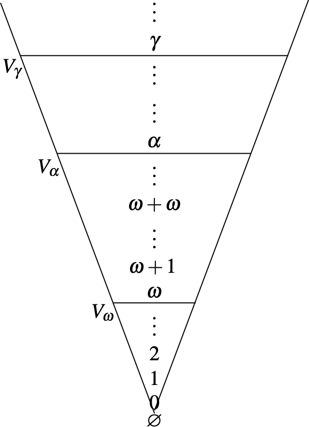
One obtains \(\{V_{\beta} : \beta \text{ is an ordinal}\}\) by repeatedly applying the power set operation at successor ordinals and by taking the union of all the previous sets at limit ordinals. In particular, \(V_{0} = \varnothing\) and
The regularity axiom implies that for every set \(x\), there exists an ordinal \(\alpha\) such that \(x \in V_{\alpha}\). For this reason, the proper class \(V = \bigcup \{V_{\beta} : \beta \text{ is an ordinal}\}\) is called the universe of sets. It follows that each set \(V_{\beta}\) is in \(V\) and that all of the axioms in ZF are true in \(V\). In addition, as one ascends the “ordinal spine,” one obtains sets \(V_{\gamma}\) of ever greater complexity that become better and better approximations to \(V\) (see above figure). This is confirmed by the reflection principle (see below) which, in essence, asserts that any statement that is true in \(V\), is also true in some set \(V_{\beta}\).
Let \(\varphi (v_{1}, \ldots , v_{n})\) be a formula in the language of set theory with free variables \(v_{1}, \ldots , v_{n}\). For any ordinal \(\alpha\) and \(x_{1}, \ldots , x_{n} \in V_{\alpha}\), we write
\((V_{\alpha}, \in) \vDash \varphi (x_{1}, \ldots , x_{n})\)
to mean that \(\varphi(x_{1}, \ldots ,x_{n})\) is true in \(V_{\alpha}\). The following theorem of ZF, due to Azriel Levy (Levy 1960) and Richard Montague (Montague 1961), implies that any specific truth that holds in \(V\) likewise holds in some initial segment \(V_{\beta}\) of \(V\); in fact, it holds in unboundedly many initial segments.
Reflection Principle: Let \(\varphi(v_{1}, \ldots, v_{n})\) be a formula and let \(\alpha\) be an ordinal. Then there is an ordinal \(\beta \) > \(\alpha\) such that, for all \(x_{1}, \ldots , x_{n} \in V_{\beta}, \varphi (x_{1}, \ldots ,x_{n})\) is true in \(V\) if and only if \((V_{\beta}, \in) \vDash \varphi (x_{1}, \ldots, x_{n})\).
As a corollary, for any finite number of formulas that hold in \(V\), the reflection principle implies that all of these formulas also hold in some \(V_{\beta}\). As noted before, there are an infinite number of axioms in ZF. Montague (Montague 1961) used the reflection principle to conclude that if ZF is consistent, then ZF is not finitely axiomatizable. Hence, ZF is not equivalent to any finite number of the axioms in ZF. This follows from Gödel’s second incompleteness theorem (see Kunen 2011, page 8), which implies that, if ZF is consistent, then one cannot prove, in ZF, the existence of a set model of ZF, that is, a set \(M\) such that \((M,\in) \vDash \varphi\), for every axiom \(\varphi\) in ZF.
7. Gödel’s Constructible Universe
As we have seen, the cumulative hierarchy of sets is constructed in stages. At successor stages, one adds all possible subsets of the previous stage and, at limit stages, one takes the union of all of the previously produced sets. To prove that the axiom of choice and the Continuum Hypothesis are consistent with ZF, Kurt Gödel (1938) constructed the “inner model” \(L\) of \(V\) commonly known as the universe of constructible sets. As we will see, \(L\) is a subclass of \(V\). The idea behind Gödel’s construction of \(L\) is to modify the cumulative hierarchy structure so that the end result will produce a (smaller) class that satisfies ZF. For any set \(X\), define \(D(X)\) to
\(D(X) = \{A \subseteq X: A\) is definable over \((X,\in)\}\)
where \(A\) is definable over \((X,\in)\) means that there are \(x_{1},\ldots,x_{n}\) in \(X\) and a formula \(\varphi(v,x_{1},\ldots,x_{n})\) such that, for all \(a\) in \(X\),
\(a \in A\) if and only if \((X,\in) \vDash \varphi (a,x_{1},\ldots,x_{n})\).
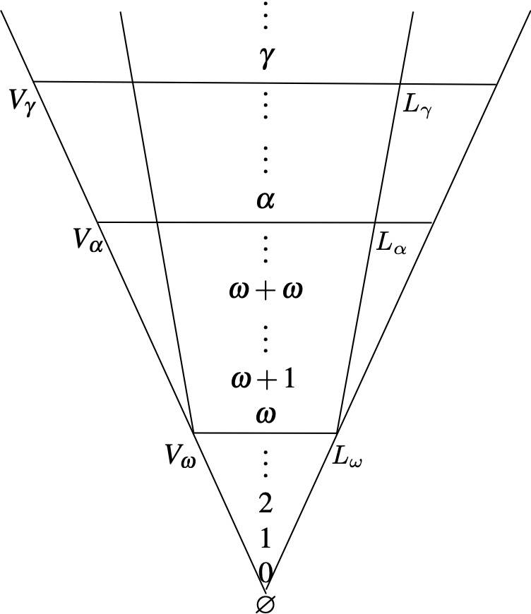
One can show, in ZF, that \(D\) is a class function (Moschovakis 2009, 8D). Using the transfinite recursion theorem and the “definable subset” operation \(D\), Gödel defined the class \(\{L_{\beta} : \beta \text{ is an ordinal}\}\) by applying the operation \(D\) at successor ordinals and by taking the union of all of the previous sets at limit ordinals. The class \(\{L_{\beta} : \beta\text{ is an ordinal}\}\) satisfies the following (see figure below):
- \(L_{0} = \varnothing\),
- \(L_{\gamma + 1} = D(L_{\gamma})\), for any ordinal \(\gamma\),
- \(L_{\beta} = \bigcup \{L_{\alpha}\) : \(\alpha \) < \(\beta\}\), for any limit ordinal \(\beta\).
Consequently, at each successor stage of the construction, one extracts only the definable subsets of the previous stage. The proper class \(L = \bigcup\{L_{\beta} : \beta\text{ is an ordinal}\}\) is called the universe of constructible sets.
Assuming ZF, Gödel proved that \(L\) satisfies ZF, the axiom of choice, and the Continuum Hypothesis (Gödel 1990). Thus, if ZF is consistent, then so is the theory ZF+AC+CH. This result does not prove that the axiom of choice and the Continuum Hypothesis are true in \(V\), but it does show that one cannot prove, in ZF, that either AC or CH is false.
The proper class \(L\) (with the \(\in\) relation restricted to \(L\)) is called an inner model, because it is a transitive class (a class that includes all of the elements of its elements), contains all of the ordinals, and satisfies all of the axioms in ZF.
Gödel’s notion of a constructible set has led to interesting and fruitful discoveries in set theory. By generalizing Gödel’s definition of \(L\), contemporary set theorists have defined a variety of inner models that have been used to establish new consistency results (Kanamori 2003, pp. 34-35). Each of these inner models contains \(L\) as a subclass, and to understand the structure of these inner models, one must be familiar with the above definition of Gödel’s constructible sets. Moreover, a penetrating investigation into the structure of \(L\) has led researchers to discover many fascinating results about \(L\) and its relationship to the universe of sets \(V\) (Jech 2003).
8. Cohen’s Forcing Technique
In 1963, the mathematician Paul Cohen introduced an extremely powerful method, called forcing, for the construction of models of Zermelo-Fraenkel set theory. A model M of set theory is a transitive collection of sets in which the ZF (ZFC) axioms are all true, denoted by M \(\vDash\) ZF (M \(\vDash\) ZFC).
As discussed in section 7, Gödel showed that one cannot prove, in ZF, that either AC or CH is false. Cohen used his forcing technique to construct a model of ZFC in which the Continuum Hypothesis is false. Hence, one cannot prove, in ZFC, that CH is true. Thus, if ZFC is consistent, then CH is undecidable in ZFC. Cohen (1963) also showed that his technique of forcing can be used to produce a model of set theory in which ZF holds and the axiom of choice is false. Thus, AC is not provable in ZF. So, if ZF is consistent, then AC is undecidable in ZF.
Cohen’s idea was to start with a given set model \(M\) of ZFC (the ground model) and extend it by adjoining a “generic” set \(G\) to \(M\) where \(G \notin M\). The resulting model \(M[G]\) (a generic extension of \(M\)) includes \(M\), contains \(G\), and satisfies ZFC. Cohen showed how to find a set \(G\) so that CH fails in \(M[G]\). In a similar manner, Cohen was able to add a new set \(G\) to \(M\) such that there is an inner model of \(M[G]\) in which ZF holds and the axiom of choice is false. For his work, Cohen was awarded the Fields Medal in 1966. This award is considered to be the “Nobel Prize” of mathematics. Gödel stated that Cohen’s forcing method was “the greatest advance in the foundations of set theory since its axiomatization” (Kanamori 2003, page 32).
The discussion in the previous paragraph about \(M\) is neither complete nor entirely correct. In order to prove that the desired generic set \(G\) exists, Cohen, in fact, had to assume that \(M\) is a countable transitive set model of ZFC. Let us do the same. A partial order is a pair \((P,\leq)\) such that \(P \neq \varnothing\) and \(\leq\) is a relation on \(P\) which is reflexive, antisymmetric, and transitive. By varying \((P,\leq)\), one can obtain generic extensions that satisfy a wide variety of statements that are consistent with ZFC. Let \((P,\leq) \in M\) be a partial order that is definable in \(M\), and suppose that, in \(M\), the definition of \((P,\leq)\) and its properties are based only on the fact that \(M \vDash ZF.\) Since \(M\) is countable, there exists a generic set \(G \subseteq P\) (Kunen 2012, Lemma IV.2.3). Let us presume that \((P,\leq)\) has the properties required to ensure that \(M[G] \vDash \varphi\), where \(\varphi\) is a sentence in the language of set theory; for example, \(\varphi\) could be “not CH.” Hence, \(M[G] \vDash\) ZFC \(+~\varphi\). Thus,
(6)
To conclude that ZFC \(+~\varphi\) is consistent, it appears that one must first show that there exists a countable transitive set model of ZFC. However, by Gödel’s second incompleteness theorem, one cannot prove, in ZFC, that such a set model exists (unless ZFC is inconsistent). Is there a way around this difficulty? Note that there are finitely many axioms in ZFC such that if just these axioms hold in \(M\), then one can still prove that \(M[G] \vDash \varphi\) (Kunen 2011).
We now discuss how the above argument used to establish (6) can be modified to correctly conclude that ZFC \(+~\varphi\) is consistent. Let \(T\) be a finite set of axioms in ZFC. Using the reflection principle, one can prove, in ZFC, that
(7)
For any finite set \(S\) of axioms in ZFC, the forcing method shows that there is a finite set \(T\) of axioms in ZFC such that \(S \subseteq T\) and
(8)
Since \(T\) is a finite set of axioms, we conclude from (7) that there is a countable transitive set model \(M\) that satisfies all of the axioms in \(T\). Therefore, by (8), there is a generic extension \(M[G]\) that satisfies \(\varphi\) and all of the axioms in \(S\). Since proofs are finite, we conclude that, in ZFC, one cannot prove \(\neg \varphi\). Hence, ZFC \(+~\varphi\) is consistent, assuming that ZFC is consistent.
Cohen’s forcing technique is very versatile and has been used to show that there are many statements, both in set theory and in mathematics, that are undecidable (or unprovable) in ZF and ZFC. For example, in mathematics, the Hahn–Banach theorem is a crucial tool used in functional analysis. The proof of this theorem uses the axiom of choice. The forcing method has been used to show that Hahn–Banach theorem is not provable in ZF alone (Jech 1974). Moreover, using forcing results and the universe of constructible sets, Saharon Shelah (1974) has shown that a famous open problem in abelian group theory (Whitehead’s Problem) is undecidable in ZFC.
As suggested earlier, since essentially all mathematical concepts can be formalized in the language of set theory, set theory offers a unifying theory for mathematics. Thus, the theorems of mathematics can be viewed as assertions about sets. Moreover, these theorems can also be proven from ZFC, the Zermelo-Fraenkel axioms together with the axiom of choice. Cohen’s forcing method clearly shows that ZFC is an incomplete theory, as there are statements that cannot be resolved in it. This motivates the following question:
What path should be taken to try to settle the Continuum Hypothesis and other undecided statements in mathematics?
In contemporary set theory, the most common answer to this question is called Gödel’s Program:
Search for new axioms, which, when added to ZFC, will determine the truth or falsity of unresolved statements.
This program was inspired by an article of Gödel’s in which he discusses the mathematical and philosophical aspects of mathematical statements that are independent of ZFC (Gödel 1947). Sections 9 and 10 will discuss two directions that this program has taken: large cardinal axioms and determinacy axioms.
9. Large Cardinal Axioms
Roughly, a large cardinal axiom is a set-theoretic statement that asserts the existence of an uncountable cardinal \(\kappa\) that satisfies a particular property that implies that there is a set \(M\) such that \((M,\in)\) is a model of ZFC; such a \(\kappa\) is called a large cardinal. Gödel’s second incompleteness theorem implies that, in ZFC, one cannot prove the existence of large cardinals. Thus, a large cardinal axiom is a “new axiom.” Most modern set theorists believe that the standard large cardinal axioms are consistent with ZFC.
Assuming ZFC, let us say that a cardinal \(\kappa\) is a strong limit cardinal if and only if, for every cardinal \(\lambda\), if \(\lambda\) < \(\kappa\), then \(2^{\lambda}\) < \(\kappa\). A cardinal \(\kappa\) is said to be inaccessible if and only if \(\kappa\) is uncountable, regular, and a strong limit cardinal. Recall that a cardinal \(\kappa\) is regular if \(\kappa\) is not the union of fewer than \(\kappa\) many sets of size each less than \(\kappa\). If \(\kappa\) is an inaccessible cardinal, then, in ZFC, one can prove that \((V_{\kappa},\in)\) is a model of ZFC (Kanamori 2003). Hence, such a \(\kappa\) is an example of a large cardinal and so, the statement “there exists an inaccessible cardinal” is a large cardinal axiom.
There are other large cardinal axioms. The description of these large cardinal axioms usually involves the concept of an elementary embedding of the universe, that is, a nontrivial truth preserving transformation from \((V,\in)\) into \((M,\in)\) where \(M\) is a transitive subclass of \(V\). A theorem of Kenneth Kunen (Jech 2003) shows that there is no nontrivial elementary embedding of the universe \(V\) into itself. Thus, for any nontrivial truth preserving transformation from \((V,\in)\) into \((M,\in)\) where \(M\) is a transitive subclass of \(V\), \(M \neq V\). More specifically, a large cardinal axiom can be expressed as asserting that there exists a nontrivial (class) function
\(j: V \rightarrow M\)
such that for each formula \(\varphi(v_{1},v_{2},\ldots,v_{n})\) (in the language of set theory) and for all elements \(x_{1},\ldots,x_{n}\) in \(V\),
\((V,\in) \vDash \varphi(x_{1},\ldots,x_{n})\) if and only if \((M,\in) \vDash \varphi(j(x_{1}),\ldots,j(x_{n}))\).
Since the embedding \(j\) is not the identity, there must be a least ordinal \(\kappa\) such that \(\kappa\) < \(j(\kappa)\). This ordinal is called the critical point of \(j\) and is denoted by \(\kappa\) = crit\((j)\). It follows that \(\kappa\) is a cardinal; indeed, \(\kappa\) is the large cardinal that is confirmed by the existence of the embedding \(j\).
A cardinal \(\kappa\) is said to be measurable if and only if there exists an embedding \(j: V \rightarrow M\) such that \(\kappa\) is the critical point of \(j\). In this case, one can prove that \(V_{\kappa+1} \subseteq M\). Therefore, there is some resemblance between \(M\) and \(V\). Increasingly stronger large cardinal axioms demand a greater agreement between \(M\) and \(V\). For example, if one requires that \(V_{\kappa+2} \subseteq M\), then one obtains a stronger large cardinal axiom. For another example, a cardinal \(\kappa\) is said to be superstrong if and only if there is a transitive class \(M\) and a nontrivial elementary embedding \(j: V \rightarrow M\) such that \(\kappa\) = crit\((j)\) and \(V_{j(\kappa)} \subseteq M\). Even stronger large cardinal axioms are obtained by requiring greater and greater resemblance between \(M\) and \(V\) (Woodin 2011).
Large cardinal axioms are statements that assert the existence of large cardinals. These axioms are widely viewed as being very promising new axioms for set theory. Large cardinal axioms do not resolve the Continuum Hypothesis but they have led mathematicians to formulate conditions under which Cantor’s hypothesis is false (Woodin 2001, p. 688). As already mentioned, one cannot prove, in ZFC, that large cardinals exist. Yet, there is very strong evidence that their existence cannot be refuted in ZFC (Maddy 1988).
10. The Axiom of Determinacy
Descriptive set theory has its origins, in the early 20th century, with the theory of real-valued functions and sets of real numbers developed by Borel, Baire, and Lebesgue. These analysts, respectively, introduced
- the hierarchy of Borel sets of real numbers,
- the Baire hierarchy of real-valued functions,
- Lebesgue measurable sets of real numbers.
Descriptive set theory extends the work of these mathematicians (Moschovakis 2009). Recall that \(\omega = \{0,1,2,3,4,\ldots\}\) is the set of natural numbers. Let \(^{\omega}\omega\) be the set of all functions from \(\omega\) to \(\omega\). The set \(^{\omega}\omega\) is denoted by \(\mathbb{R}\) and is called Baire Space. \(\mathbb{R}\) is often referred to the set of reals; and if \(x \in \mathbb{R}\), then \(x\) is called a real. \(\mathbb{R}\) is regarded as a topological space by giving it the product topology, using the discrete topology on \(\omega\). The space \(\mathbb{R}\) is homeomorphic to the set of irrational numbers which is a subspace of the set of real numbers (Moschovakis 2009).
Descriptive set theory is a branch of set theory that uses set theoretic tools to investigate the structure of definable sets and functions over \(\mathbb{R}\). One can identify the level of complexity of such definable sets of reals (Moschovakis 2009). Thus, there is a natural hierarchy on the definable subsets of \(\mathbb{R}\), which, in increasing order of complexity, is called the projective hierarchy.
As a result of Gödel’s and Cohen’s work, it has been shown that many questions in descriptive set theory are not decidable in axiomatic set theory. For example, in 1938, Gödel showed that in \(L\), the universe of constructible sets, there are projective sets of reals that are not Lebesgue measurable. In 1970, using the method of forcing, Robert Solovay showed that if there is an inaccessible cardinal, then ZFC is consistent with the statement that every projective set is Lebesgue measurable. Thus, one can neither prove nor disprove, in ZFC, the Lebesgue measurability of projective sets. Hence, in ZFC, the theory of projective sets is incomplete. For this reason, modern descriptive set theory focuses on new axioms; one such axiom concerns infinite games.
Gale and Stewart (1953) introduced the general concept of an infinite game of perfect information and began the study of these games. Other mathematicians then pursued this subject and discovered that it can be used to resolve problems in descriptive set theory.
We now turn to a description of infinite games and strategies. For each \(A \subseteq \mathbb{R}\), we associate a two-person infinite game on \(\omega\) with payoff \(A\), denoted by \(G_{A}\), where players I and II alternately choose natural numbers \(a_{i}\) in the order given in the diagram:

After completing an infinite number of moves, the players produce the real
\(x =\) ⟨\(a_{0},a_{1},a_{2},\ldots\)⟩.
Player I is said to win if \(x \in A\), otherwise player II is said to win. As each player is aware of all the previous moves before making a next move, the game is called a game of perfect information. The game \(G_{A}\) is said to be determined if and only if either player has a “winning strategy,” that is, a function that ensures the player will win the game regardless of how the other player makes his or her moves. The Axiom of Determinacy (AD) is a regularity hypothesis about such games that states: For all \(A \subseteq \mathbb{R}\), the game \(G_{A}\) is determined.
In the theory ZF+AD, one can resolve many open questions about the sets of real numbers. For example, one can prove Cantor’s original form of the continuum hypothesis: Every uncountable set of real numbers has the same cardinality as the full set of real numbers.
Moreover, it has been shown that the axiom of choice implies that AD is false; that is, using the axiom of choice, one can construct a set of reals \(A\) such that the game \(G_{A}\) is not determined. Thus, the axiom of determinacy is incompatible with the axiom of choice. However, it is not clear that one can establish, without the axiom of choice, the existence of a set of reals \(A\) such that the game \(G_{A}\) is not determined (Moschovakis 2009). Moreover, there are weaker versions of AD that are compatible with ZF together with a weaker choice principle called the axiom of dependent choices.
Axiom of Dependent Choices (DC). Let \(R\) be a relation on a nonempty set \(A\). Suppose that for all \(x \in A\) there is a \(y \in A\) such that \(R(x,y)\). Then there exists a function \(f: \omega \rightarrow A\) such that, for all \(n \in \omega\), \(R(f(n),f(n+1))\).
Many mathematicians working in descriptive set theory operate within the background theory ZF+DC and the following determinacy axiom: For every projective set \(A\), the game \(G_{A}\) is determined. This axiom is denoted by PD (projective determinacy). Under the theory ZF+DC+PD, the classic open questions about projective sets have been successfully addressed (Moschovakis 2009). In particular, this theory implies that all projective sets are Lebesgue measurable.
Generalizing the construction of the inner model \(L\), one can construct the inner model \(L(\mathbb{R})\), the smallest inner model that contains all the ordinals and all the reals. The set \(\wp(\mathbb{R}) \cap L(\mathbb{R})\) can be viewed as a natural extension of the projective sets. The determinacy hypothesis denoted by AD\(^{L(\mathbb{R})}\), asserts that AD holds in \(L(\mathbb{R})\). Since the inner model \(L(\mathbb{R})\) contains all of the projective sets, the assumption AD\(^{L(\mathbb{R})}\) implies PD.
There are very deep results that connect determinacy hypotheses and large cardinal axioms. In 1988, Martin and Steel, working in ZFC, identified a large cardinal axiom that implies PD. By assuming a stronger large cardinal axiom, Woodin, within ZFC, was able to prove that AD\(^{L(\mathbb{R})}\) holds and so, \(L(\mathbb{R})\) satisfies ZF+AD. Moreover, PD and AD\(^{L(\mathbb{R})}\), individually, imply the consistency of certain large cardinal axioms (Kanamori 2003). Investigating the relationships between determinacy hypotheses and large cardinals has become an important component of modern set theory.
11. Concluding Remarks
Set Theory is a rich and beautiful branch of mathematics whose fundamental concepts permeate all branches of mathematics. It is a most extraordinary fact that all standard mathematical objects can be defined as sets. For example, the natural numbers and the real numbers can be constructed within set theory. In addition, algebraic structures, functional spaces, vector spaces, and topological spaces can be viewed as sets in the universe of sets \(V\). Consequently, mathematical theorems can be regarded as statements about sets. These theorems can also be proven from ZFC, the axioms of set theory. Thus, mathematics can be embedded into set theory.
Since all of conventional mathematics can be developed within set theory, one can view certain results in set theory as being part of metamathematics, the field of study within mathematics that uses mathematical tools to investigate the nature and power of mathematics. For example, using the forcing technique and inner models, it has been shown that there are mathematical statements that cannot be proven or disproven in ZFC. Thus, when a particular mathematical statement is unresolved, set theory can sometimes show that there is neither a proof nor a refutation of the statement in ZFC. As noted above, this situation has inspired the search for new set theoretic axioms.
Of course, the fact that set theory offers a foundation for mathematics indicates that set theory is a very important branch of mathematics. However, the concepts and techniques developed within set theory demonstrate that, in itself, set theory is a deep and exciting branch of mathematics with significant applications to other areas of mathematics. This success has inspired some philosophers of mathematics to direct their attention to the philosophy of set theory and the search for new axioms (Maddy 1988a, 1988b, 2011).
12. References and Further Reading
a. Primary Sources
- Banach, S. and Tarski, A. 1924. “Sur la décomposition des ensembles de points en parties respectivement congruentes,” Fund. Math., 6, pp. 244–277.
- Cantor, Georg. 1874. “Über eine Eigenschaft des Inbegriffes aller reellen algebraischen Zahlen,” Journal fur die reine und angewandte Mathematik (Crelle). 77, 258–262.
- Cohen, Paul J. 1963. The independence of the axiom of choice. Mimeographed.
- Cohen, Paul J. 1963a. “The independence of the continuum hypothesis I.” Proceedings of the U.S. National Academy of Sciences 50, 1143-48.
- Cohen, Paul J. 1964. “The independence of the continuum hypothesis II.” Proceedings of the U.S. National Academy of Sciences 51, 105-110.
- Cohen, Paul J. 1966. Set Theory and the Continuum Hypothesis, New York: Benjamin.
- Cunningham, Daniel W. 2016. Set Theory: A First Course, New York: Cambridge University Press.
- Dauben, Joseph W. 1979. Georg Cantor: his mathematics and philosophy of the infinite, Cambridge, Mass., Harvard University Press; reprinted: Princeton, Princeton University Press, 1990.
- Dunham, William. 1990. Journey Through Genius: The Great Theorems of Mathematics (1st ed.). John Wiley and Sons.
- Gale, D. and Stewart, F.M. 1953. “Infinite games with perfect information,“ Annals of Math. Studies, vol. 28, pp. 245–266.
- Gödel, Kurt. 1947. “What is Cantor’s Continuum Problem?,” American Mathematical Monthly, vol. 54, pp. 515-525.
- Gödel, Kurt. 1986. Collected Works, Volume I: Publications 1929–1936, (Solomon Feferman, editor-in-chief), Oxford University Press, New York.
- Gödel, Kurt. 1990. Collected Works, Volume II: Publications 1938–1974, (Solomon Feferman, editor-in-chief), Oxford University Press, New York.
- Gödel, Kurt. 1995. Collected Works, Volume III: Unpublished Essays and Lectures, (Solomon Feferman, editor-in-chief), Oxford University Press, New York.
- Hilbert, David. 1923. On the infinite. Reprinted in the Philosophy of Mathematics: Selected Readings, 1983, edited by Paul Benacerraf and Hilary Putnam, pp. 83-201.
- Jech, Thomas. 2003. Set theory. Third Edition, New York: Springer.
- Jech, Thomas. 1973. The Axiom of Choice, North-Holland Publishing Company, Studies in logic and the foundations of mathematics, vol. 75, Amsterdam.
- Kanamori A. 2003. The Higher Infinite. Perspectives in Mathematical Logic. Second edition. Berlin: Springer.
- Kanamori A. 2012. Set theory from Cantor to Cohen, a book chapter in: Handbook of the History of Logic: Sets and Extensions in the Twentieth Century. Volume editor: Akihiro Kanamori. General editors: Dov M. Gabbay, Paul Thagard and John Woods. Elsevier BV.
- Kunen, Kenneth. 2009. The Foundations of Mathematics. Studies in Logic, vol. 19. London: College Publications.
- Kunen, Kenneth. 2011. Set Theory. Studies in Logic, vol. 34. London: College Publications.
- Lévy, Azriel. 1960. “Axiom schemata of strong infinity in axiomatic set theory,” Pacific Journal of Mathematics, 10, pp. 223–238.
- Maddy, Penelope H. 1988a. “Believing the axioms I.” The Journal of Symbolic Logic, 53(2), 481–511.
- Maddy, Penelope H. 1988b. “Believing the axioms II.” The Journal of Symbolic Logic, 53(3), 736–764.
- Maddy, Penelope H. 2011. Defending the axioms. On the philosophical foundations of set theory. Oxford: Oxford University Press.
- Montague, Richard M. 1961. Fraenkel’s addition to the axioms of Zermelo. Essays on the foundations of mathematics, dedicated to A. A. Fraenkel on his seventieth anniversary, edited by Y. Bar-Hillel, E. I. J. Poznanski, M. O. Rabin, and A. Robinson for The Hebrew University of Jerusalem, Magnes Press, Jerusalem, and North-Holland Publishing Company, Amsterdam, pp. 91–114.
- Moore, Gregory H. 2012. Zermelo’s Axiom of Choice: Its Origins, Development, and Influence. Mineola, NY: Dover Publications. Reprint of the 1982 original published by Springer.
- Moschovakis, Yiannis. 2009. Descriptive Set Theory, 2nd edition, vol. 155 of Mathematical Surveys and Monographs, American Mathematical Society, Providence, 2009.
- Solovay, Robert. 1970. “A model of set theory in which every set is Lebesgue measurable.” Annals of Mathematics, vol. 92, 1–56.
- Shelah, Saharon. 1974. “Infinite abelian groups, Whitehead problem and some constructions.” Israel J. Math, vol. 18, 243–256.
- Woodin, Hugh. 2001. “The Continuum Hypothesis, Part II.” Notices of the American Mathematical Society, vol. 48, no. 7.
- Woodin, Hugh. 2011. Infinity, a book chapter in: Infinity: New Research Frontiers. Cambridge: Cambridge University Press.
- Zermelo, Ernst. 2010. Collected Works. Gesammelte Werke. Volume I: Set Theory, Miscellania. Mengenlehre, Varia, edited by H.-D. Ebbinghaus and A. Kanamori, Springer, Berlin and Heidelberg, xxiv + 654 pp.
b. Secondary Sources
- Ebbinghaus, Heinz-Dieter. 2007. Ernst Zermelo. An Approach to His Life and Work. Berlin: Springer. In cooperation with Volker Peckhaus.
- Enderton, Herbert B. 1977. Elements of Set Theory. New York: Academic Press.
- Enderton, Herbert B. 2001. A Mathematical Introduction to Logic. 2nd edn. Burlington, MA: Harcourt/Academic Press.
- Feferman, Solomon, Parsons, Charles and Simpson, Steven G. (Eds.). 2010. Kurt Gödel: essays for his centennial. Cambridge: Cambridge University Press.
- Halmos, Paul R. 1974. Naïve Set Theory. New York: Springer. Reprint of the 1960 edition published by Van Nostrand.
- Hauser, Kai. 2006. “Gödel’s Program Revisited Part I: The Turn to Phenomenology.” Bulletin of Symbolic Logic, 12(4), 529–590.
- Heller, Michael and Woodin, Hugh. (Eds.). 2011. Infinity: New Research Frontiers. Cambridge: Cambridge University Press.
- Kanamori, Akihiro. 2012. “In praise of replacement.” Bulletin of Symbolic Logic, 18(1), 46–90.
- Levy, Azriel. 2002. Basic Set Theory. Mineola, NY: Dover Publications. Reprint of the 1979 original published by Springer.
- Moschovakis, Yiannis. 2006. Notes on Set Theory. 2nd edition. Undergraduate Texts in Mathematics. New York: Springer.
- Potter, Michael. 2004. Set theory and Its Philosophy. New York: Oxford University Press.
c. Internet Sources
- Mathematical Induction
- Logic and set theory around the world
- Directory of links on logic and foundations of mathematics
- Gödel’s incompleteness theorems
Author Information
Daniel Cunningham
Email: cunnindw@buffalostate.edu
State University of New York Buffalo State
U. S. A.